Phase Modulator

The electro-optic phase modulator is the elementary building block behind most modulators: on its own it encodes information in the optical phase, and combined with interferometers or resonators it becomes an intensity modulator. The PhaseModTimeStepper models a uniform (lumped) phase modulator of length \(\ell\) for time-domain simulations, with the driving voltage applied through an electrical port. The induced phase shift and optical loss follow

\[\Delta \phi = \frac{\pi V \ell}{V_{\pi L}} + k_2 V^2 \ell + k_3 V^3 \ell \qquad L = \left( L_p + \frac{\mathrm{d} L_p}{\mathrm{d} V} V + \frac{\mathrm{d}^2 L_p}{\mathrm{d} V^2} V^2 \right) \ell\]

where \(V_{\pi L}\) is the electro-optic phase coefficient (so a modulator of length \(\ell\) has \(V_\pi = V_{\pi L} / \ell\)), \(k_2\) and \(k_3\) add nonlinear phase terms, and the loss \(L\) combines the propagation loss \(L_p\) with voltage-dependent absorption terms. The electrical input amplitude \(A\) is converted to the driving voltage as \(V = \Re \lbrace A \rbrace \sqrt{Z_0}\). The model also includes an optional first-order low-pass filter on the electrical input (f_3dB) and group delay through the optical path (n_group).

This guide characterizes the phase and loss laws, shows the optical sidebands created by sinusoidal phase modulation, measures the electrical bandwidth limit, and finally assembles a Mach-Zehnder intensity modulator around the phase modulator.

Setup

import matplotlib.pyplot as plt
import numpy as np
from scipy.special import jv
import photonforge as pf
import photonforge.abstract as pfa

viewer = pf.live_viewer.LiveViewer()

LiveViewer started at http://localhost:56820

tech = pf.basic_technology()
pf.config.default_technology = tech

lda0 = 1.55
f0 = pf.C_0 / lda0
z0 = 50.0
time_step = 1e-12

Phase Shift vs Voltage

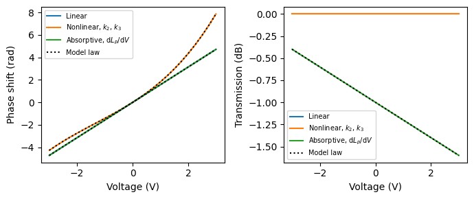
The abstract phase_modulator component has two optical ports, P0 and P1, and one electrical drive port, E0. We use a 5 mm long modulator with \(V_{\pi L} = 1\) V·cm, a typical value for silicon depletion-mode phase shifters, giving \(V_\pi = V_{\pi L} / \ell = 2\) V.

length = 5000.0
v_pil = 10000.0
v_pi = v_pil / length

modulator = pfa.phase_modulator(length=length, v_piL=v_pil)
viewer(modulator)

To characterize the static transfer we drive E0 with a constant voltage from a signal_source, an abstract signal generator based on the WaveformTimeStepper. Setting its amplitude to zero leaves only the constant offset, which, like all electrical signals, is specified as a wave amplitude, \(V / \sqrt{Z_0}\).

We sweep the DC voltage, record the phase of the output envelope relative to the unbiased case, and repeat for a modulator with nonlinear coefficients \(k_2\) and \(k_3\). A modulator with voltage-dependent absorption (dloss_dv), typical of carrier-based devices, shows its transmission change alongside. The corresponding analytic laws are plotted as dotted lines for reference.

variants = {
    "Linear": {},
    "Nonlinear, $k_2$, $k_3$": {"k2": 4e-5, "k3": 1e-5},
    "Absorptive, d$L_p$/d$V$": {"propagation_loss": 2e-4, "dloss_dv": 4e-5},
}

voltages = np.linspace(-3, 3, 25)
num_steps = 200

fig, (ax1, ax2) = plt.subplots(1, 2, figsize=(7, 3), tight_layout=True)
for label, kwargs in variants.items():
    modulator_dc = pfa.phase_modulator(length=length, v_piL=v_pil, **kwargs)
    source = pfa.signal_source(amplitude=0, offset=0)
    link = pf.Component("dc_link")
    laser_ref = link.add_reference(pfa.cw_laser(power=1e-3))
    modulator_ref = link.add_reference(modulator_dc)
    source_ref = link.add_reference(source)
    modulator_ref.connect("P0", laser_ref["P0"])
    source_ref.connect("E0", modulator_ref["E0"])
    link.add_port(modulator_ref["P1"], "out")
    link.add_model(pf.CircuitModel(), "Circuit")

    phases = []
    transmission = []
    for voltage in voltages:
        source.update(offset=voltage / np.sqrt(z0))
        time_stepper = link.setup_time_stepper(
            time_step=time_step, carrier_frequency=f0, show_progress=False
        )
        a = time_stepper.step(steps=num_steps, time_step=time_step, show_progress=False)["out@0"]
        phases.append(np.angle(a[-1]))
        transmission.append(10 * np.log10(np.abs(a[-1]) ** 2 / 1e-3))
    phases = np.unwrap(np.array(phases))
    ax1.plot(voltages, phases - phases[len(voltages) // 2], label=label)
    ax2.plot(voltages, transmission, label=label)

k2, k3 = variants["Nonlinear, $k_2$, $k_3$"]["k2"], variants["Nonlinear, $k_2$, $k_3$"]["k3"]
loss_p, dloss = variants["Absorptive, d$L_p$/d$V$"]["propagation_loss"], variants["Absorptive, d$L_p$/d$V$"]["dloss_dv"]
ax1.plot(voltages, np.pi * voltages / v_pi, "k:", label="Model law")
ax1.plot(voltages, np.pi * voltages / v_pi + k2 * voltages**2 * length + k3 * voltages**3 * length, "k:")
ax2.plot(voltages, -(loss_p + dloss * voltages) * length, "k:", label="Model law")
ax1.set(xlabel="Voltage (V)", ylabel="Phase shift (rad)")
ax2.set(xlabel="Voltage (V)", ylabel="Transmission (dB)")
ax1.legend(fontsize=7)
_ = ax2.legend(fontsize=7)

Sinusoidal Modulation and Optical Sidebands

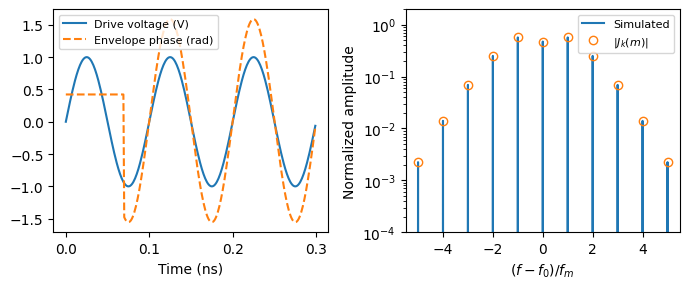
Driving the phase with a sine wave, \(\Delta \phi (t) = m \sin(2 \pi f_m t)\), produces the classic phase-modulation spectrum: discrete sidebands at multiples of \(f_m\) around the carrier, with amplitudes given by Bessel functions of the modulation index \(m\),

\[a(t) = \sqrt{P} \, e^{j m \sin(2 \pi f_m t)} = \sqrt{P} \sum_{k=-\infty}^{\infty} J_k(m) \, e^{j k 2 \pi f_m t}\]

We drive the modulator with a 1 V amplitude sine at 10 GHz, giving \(m = \pi V_m / V_\pi = \pi / 2\). A monitor placed on the modulator’s electrical port records the voltage that actually drives it (the drive appears in the incoming direction, with the - suffix in the monitor key). After removing the static propagation phase of the waveguide, the extracted envelope phase follows the drive. The analytic sideband amplitudes \(\lvert J_k(m) \rvert\) are overlaid on the simulated spectrum for comparison.

f_m = 10e9
v_m = 1.0
m_index = np.pi * v_m / v_pi

source = pfa.signal_source(frequency=f_m, amplitude=v_m / np.sqrt(z0))
link = pf.Component("sideband_link")
laser_ref = link.add_reference(pfa.cw_laser(power=1e-3))
modulator_ref = link.add_reference(modulator)
source_ref = link.add_reference(source)
modulator_ref.connect("P0", laser_ref["P0"])
source_ref.connect("E0", modulator_ref["E0"])
link.add_port(modulator_ref["P1"], "out")
link.add_model(pf.CircuitModel(), "Circuit")

num_steps = 20000
t = np.arange(num_steps) * time_step

time_stepper = link.setup_time_stepper(
    time_step=time_step,
    carrier_frequency=f0,
    time_stepper_kwargs={"monitors": {"drive": modulator_ref["E0"]}},
)
output = time_stepper.step(steps=num_steps, time_step=time_step)
a = output["out@0"]
drive_voltage = np.real(output["drive@0-"]) * np.sqrt(z0)

settled = slice(num_steps // 2, None)
spectrum = np.abs(np.fft.fftshift(np.fft.fft(a[settled]))) / len(a[settled]) / np.sqrt(1e-3)
freq_offset = -np.fft.fftshift(np.fft.fftfreq(len(a[settled]), time_step))
order = np.argsort(freq_offset)
orders = np.arange(-5, 6)

fig, (ax1, ax2) = plt.subplots(1, 2, figsize=(7, 3), tight_layout=True)
window = slice(0, 300)
phase_trace = np.angle(a[window])
ax1.plot(t[window] * 1e9, drive_voltage[window], label="Drive voltage (V)")
ax1.plot(t[window] * 1e9, phase_trace - phase_trace.mean(), "--", label="Envelope phase (rad)")
ax1.set(xlabel="Time (ns)")
ax1.legend(fontsize=8)
ax2.semilogy(freq_offset[order] / f_m, spectrum[order], label="Simulated")
ax2.semilogy(orders, np.abs(jv(orders, m_index)), "o", fillstyle="none", label="$|J_k(m)|$")
ax2.set(xlabel="$(f - f_0) / f_m$", ylabel="Normalized amplitude", xlim=(-5.5, 5.5), ylim=(1e-4, 2))
_ = ax2.legend(fontsize=8)

Electrical Bandwidth

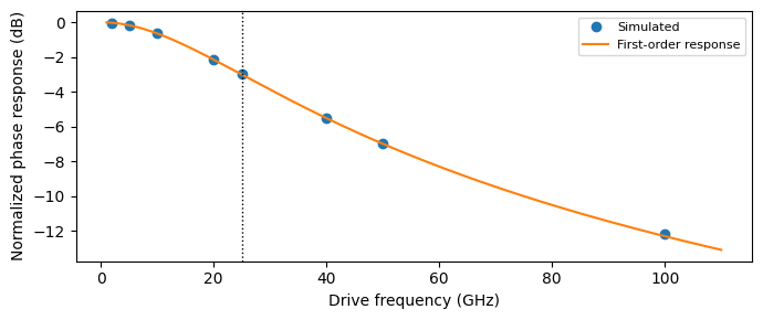
A positive f_3dB inserts a first-order low-pass filter on the electrical drive, modeling the finite bandwidth of the modulator electrodes and junction. To see its effect, we set \(f_{3\mathrm{dB}} = 25\) GHz, sweep the drive frequency with a small amplitude, and extract the modulation index at each point directly from the envelope phase. Because the components are parametric, the same circuit is updated in place at every step of the sweep. The analytic first-order response \(1 / \sqrt{1 + (f_m / f_{3\mathrm{dB}})^2}\) is plotted with the simulated points.

f_3db = 25e9
v_small = 0.2
modulator.update(f_3dB=f_3db)

drive_freqs = np.array([2e9, 5e9, 10e9, 20e9, 25e9, 40e9, 50e9, 100e9])
num_steps = 10000
t = np.arange(num_steps) * time_step
settled = slice(num_steps // 2, None)

measured = []
for drive_freq in drive_freqs:
    source.update(frequency=drive_freq, amplitude=v_small / np.sqrt(z0))
    time_stepper = link.setup_time_stepper(
        time_step=time_step, carrier_frequency=f0, show_progress=False
    )
    a = time_stepper.step(steps=num_steps, time_step=time_step, show_progress=False)["out@0"]
    phase = np.unwrap(np.angle(a))[settled]
    tone = 2 * np.abs(np.mean((phase - phase.mean()) * np.exp(-2j * np.pi * drive_freq * t[settled])))
    measured.append(tone / (np.pi * v_small / v_pi))

freq_fine = np.linspace(1e9, 110e9, 300)
fig, ax = plt.subplots(figsize=(7, 3), tight_layout=True)
ax.plot(drive_freqs / 1e9, 20 * np.log10(measured), "o", label="Simulated")
ax.plot(freq_fine / 1e9, -10 * np.log10(1 + (freq_fine / f_3db) ** 2), label="First-order response")
ax.axvline(f_3db / 1e9, color="k", linestyle=":", linewidth=1)
ax.set(xlabel="Drive frequency (GHz)", ylabel="Normalized phase response (dB)")
_ = ax.legend(fontsize=8)

_ = modulator.update(f_3dB=0)

Intensity Modulation: Mach-Zehnder

Phase is invisible to a photodiode, so on its own the phase modulator does not change the detected power. Embedding it in an interferometer converts phase to intensity. We build a Mach-Zehnder modulator from two 3 dB directional_coupler components, with the driven phase modulator in one arm. An identical modulator with its electrical port closed by an electrical_termination sits in the other arm, so both arms share the same optical path length and the interferometer is balanced at zero bias.

Because abstract components are schematic symbols, the two arms cannot always be closed geometrically. The second arm is connected with add_virtual_connection, which forces a netlist connection between ports regardless of their positions in the layout.

Sweeping the bias voltage traces the interferometric transfer function at the detector, shown together with its analytic form

\[I(V) = \frac{R P}{2} \left[ 1 - \cos\left( \frac{\pi V}{V_\pi} \right) \right]\]

responsivity = 0.8

source_mzm = pfa.signal_source(amplitude=0, offset=0)
mzm = pf.Component("mzm")
splitter_ref = mzm.add_reference(pfa.directional_coupler())
combiner_ref = mzm.add_reference(pfa.directional_coupler())
laser_ref = mzm.add_reference(pfa.cw_laser(power=1e-3))
modulator_ref = mzm.add_reference(modulator)
reference_arm_ref = mzm.add_reference(pfa.phase_modulator(length=length, v_piL=v_pil))
source_ref = mzm.add_reference(source_mzm)
photodiode_ref = mzm.add_reference(pfa.photodiode(responsivity=responsivity, seed=0))
input_term_ref = mzm.add_reference(pfa.optical_termination())
output_term_ref = mzm.add_reference(pfa.optical_termination())
electrical_term_ref = mzm.add_reference(pfa.electrical_termination())

laser_ref.connect("P0", splitter_ref["P0"])
input_term_ref.connect("P0", splitter_ref["P1"])
modulator_ref.connect("P0", splitter_ref["P2"])
source_ref.connect("E0", modulator_ref["E0"])
combiner_ref.connect("P0", modulator_ref["P1"])
reference_arm_ref.connect("P0", splitter_ref["P3"])
electrical_term_ref.connect("E0", reference_arm_ref["E0"])
mzm.add_virtual_connection(reference_arm_ref, "P1", combiner_ref, "P1")
photodiode_ref.connect("P0", combiner_ref["P2"])
output_term_ref.connect("P0", combiner_ref["P3"])
mzm.add_port(photodiode_ref["E0"])
mzm.add_model(pf.CircuitModel(), "Circuit")

bias_voltages = np.linspace(-4, 4, 33)
num_steps = 300
detected = []
for voltage in bias_voltages:
    source_mzm.update(offset=voltage / np.sqrt(z0))
    time_stepper = mzm.setup_time_stepper(
        time_step=time_step, carrier_frequency=f0, show_progress=False
    )
    v_out = np.real(
        time_stepper.step(steps=num_steps, time_step=time_step, show_progress=False)["E0@0"]
    ) * np.sqrt(z0)
    detected.append(v_out[100:].mean())

i_max = responsivity * 1e-3
fig, ax = plt.subplots(figsize=(7, 3), tight_layout=True)
ax.plot(bias_voltages, np.array(detected) * 1e3, "o", markersize=4, label="Simulated")
ax.plot(bias_voltages, i_max * (1 - np.cos(np.pi * bias_voltages / v_pi)) / 2 * 1e3, label="Analytic")
ax.axvline(v_pi / 2, color="k", linestyle=":", linewidth=1, label="Quadrature")
ax.set(xlabel="Bias voltage (V)", ylabel="Detected voltage (mV)")
_ = ax.legend(fontsize=8)

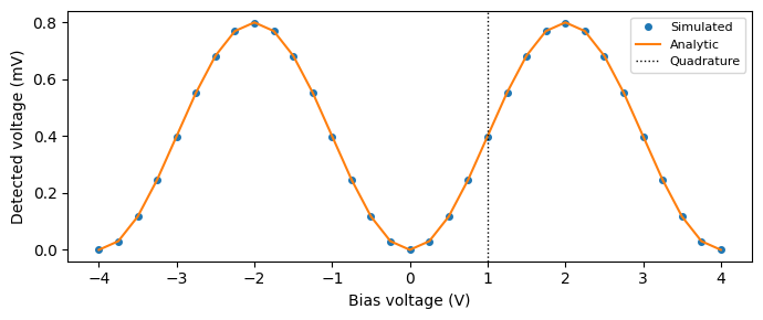
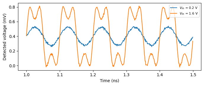
At quadrature (\(V = V_\pi / 2\), the point of maximum slope), a small drive produces a linear replica of the electrical signal in the detected power. Driving harder pushes the interferometer into the nonlinear parts of its transfer function, and the output clips as it approaches the transmission extremes.

f_m = 10e9
num_steps = 2000
t = np.arange(num_steps) * time_step

fig, ax = plt.subplots(figsize=(7, 3), tight_layout=True)
for v_amp in [0.2, 1.6]:
    source_mzm.update(
        frequency=f_m, amplitude=v_amp / np.sqrt(z0), offset=v_pi / 2 / np.sqrt(z0)
    )
    time_stepper = mzm.setup_time_stepper(
        time_step=time_step, carrier_frequency=f0, show_progress=False
    )
    v_out = np.real(
        time_stepper.step(steps=num_steps, time_step=time_step, show_progress=False)["E0@0"]
    ) * np.sqrt(z0)
    ax.plot(t[1000:1500] * 1e9, v_out[1000:1500] * 1e3, label=f"$V_m$ = {v_amp} V")

ax.set(xlabel="Time (ns)", ylabel="Detected voltage (mV)")
_ = ax.legend(fontsize=8, loc="upper right")

Summary

• pfa.phase_modulator implements the phase law \(\Delta \phi = \pi V \ell / V_{\pi L} + k_2 V^2 \ell + k_3 V^3 \ell\) with optional voltage-dependent loss; the drive voltage comes from the electrical port as \(V = \Re \lbrace A \rbrace \sqrt{Z_0}\).

• Sinusoidal phase modulation creates Bessel sidebands \(J_k(m)\) at multiples of the drive frequency, a convenient calibration of the modulation index.

• f_3dB adds a first-order low-pass on the electrical drive to model finite electrode bandwidth, and n_group sets the optical group delay through the device.

• Interferometers convert phase to intensity: two directional couplers, the driven modulator, and a matched reference arm form a Mach-Zehnder modulator with the expected raised-cosine transfer function and quadrature operation.

• Virtual connections (add_virtual_connection) close circuit topologies that cannot be drawn geometrically with schematic symbols.

• The sources and detector used here are described by the CWLaserTimeStepper and PhotodiodeTimeStepper.