Analytic Data Models Overview

PhotonForge data models are analytic, frequency domain S-matrix models attached to a component with add_model. Instead of running a mode, FDTD, or EME solver, the S matrix is built directly from a few user-supplied coefficients. They are ideal for:

• Black-box devices: represent a foundry PDK cell or a device known only by its specifications (insertion loss, splitting ratio, isolation).

• Fast circuit prototyping: get a full circuit running with CircuitModel before any physical simulation exists, then swap in solver-based models later.

• Idealized references: compare a real (simulated) device against its lossless ideal.

This guide covers the 10 built-in data models, ordered by port count: TerminationModel, TwoPortModel, WaveguideModel, IsolatorModel, PowerSplitterModel, CirculatorModel, PolarizationBeamSplitterModel, PolarizationSplitterRotatorModel, CrossingModel, and DirectionalCouplerModel.

Choosing a model at a glance

Model	Ports	Reciprocal	Key coefficients	Typical use
TerminationModel	1	n/a	r	Terminate unused ports; mirrors
TwoPortModel	2	yes	t, r0, r1 (+ phase)	Generic 2-port: attenuator, filter, fitted block
WaveguideModel	2	yes	n_complex, length (auto)	Routing waveguides; automatic mode solving
IsolatorModel	2	no	t, i, r0, r1	Isolators, direction-dependent loss
PowerSplitterModel	3	yes	t, i, r0, r1	Y-branch, 1×2 MMI
CirculatorModel	3	no	t, i, r	Circulators, reflection routing
PolarizationBeamSplitterModel	3 (2-mode)	yes	t1, t2, i, r0 to r2	PBS without rotation
PolarizationSplitterRotatorModel	3 (4 or 6 logical)	yes	s00 to s55	PSR with TM to TE rotation
CrossingModel	4	yes	t, x, r (+ phase)	Waveguide crossings
DirectionalCouplerModel	4	yes	c (auto t), i, r (+ phase)	Couplers, ring bus coupling

import matplotlib.pyplot as plt
import numpy as np
import photonforge as pf

Shared conventions

• Coefficients are complex amplitudes, not powers. A 3 dB power split is an amplitude of \(1/\sqrt{2} \approx 0.7071\), and a 0.5 dB insertion loss is 10**(-0.5 / 20).

• Port ordering: the ports argument lists the component port names that map to the rows and columns of the S matrix. If omitted, the sorted list of the component’s port names is used. Pass it explicitly whenever the sorted order is not the intended one: this is the most common source of wiring bugs.

• Multimode ports: pass a sequence of coefficients, one per mode. Mixed-mode coefficients are always 0 in these models (except in the polarization splitter rotator, where they are explicit arguments).

• Dispersion: any coefficient can be an Interpolator (frequency to value) or a 2D array of shape (M, N), with M the number of modes and N the number of frequencies used in the S matrix computation. Both are demonstrated in the frequency-dependent coefficients section.

• Reciprocity and passivity are up to the user: the models use exactly the values provided (only the circulator and isolator are intentionally non-reciprocal). A non-passive matrix can destabilize time domain co-simulation.

Additionally, TwoPortModel, CrossingModel, and DirectionalCouplerModel include a built-in propagation phase to model first-order dispersion:

\[\phi = \frac{2 \pi l_p}{c_0} \left[ n_\text{eff} f_0 + n_\text{group} (f - f_0) \right]\]

controlled by propagation_length (\(l_p\)), n_eff, n_group (defaults to n_eff), and reference_frequency (\(f_0\), defaults to the central frequency of the sweep, so pin it explicitly for reproducible phase).

Data models ignore layout geometry completely, so every model provides a black_box_component method that creates a component with the correct number of ports and the model already attached. Combined with virtual_port_spec, which creates a port specification with no path profile, complete circuits can be modeled before any layout exists (schematic-driven design). Setting the port specification in config.default_kwargs makes it the default for all black-box components. A small helper prints the non-zero S matrix elements in the demonstrations below.

tech = pf.basic_technology()
pf.config.default_technology = tech
pf.config.default_kwargs["port_spec"] = pf.virtual_port_spec()

lda_ref = 1.55
f_ref = pf.C_0 / lda_ref
frequencies = np.array([f_ref])


def show_nonzero(s_matrix):
    for (port_in, port_out), value in sorted(s_matrix.elements.items()):
        magnitude = abs(value[0])
        if magnitude > 1e-9:
            print(
                f"{port_in} -> {port_out}: {magnitude:.4f}, {np.angle(value[0]):+.4f} rad"
            )

One-port model

TerminationModel

The simplest model: a 1-port device with reflection coefficient r.

\[S = \begin{bmatrix} r \end{bmatrix}\]

The default r=0 is a perfectly matched (absorbing) load, used to terminate unused ports so that circuit solves do not leave them floating. Setting r=1 (or -1) gives an ideal mirror, and any complex value gives a lossy or phased reflector.

mirror = pf.TerminationModel(r=-1).black_box_component(name="mirror")

show_nonzero(mirror.s_matrix(frequencies))

P0@0 -> P0@0: 1.0000, +3.1416 rad

Two-port models

TwoPortModel

A generic reciprocal 2-port with transmission t in both directions, independent reflections r0 and r1, and the built-in dispersion phase:

\[\begin{split}S = \begin{bmatrix} r_0 & t \\ t & r_1 \end{bmatrix} e^{j \phi}\end{split}\]

This is the general purpose “anything with an input and an output” model: attenuators, filters, phase or delay sections, or a block fitted to measured S-parameters. It is classification-agnostic, so it also works on electrical ports.

The example below is a 1 dB attenuator that also carries the propagation phase of a 100 μm dispersive section.

attenuator = pf.TwoPortModel(
    t=10 ** (-1 / 20),
    propagation_length=100.0,
    n_eff=2.4,
    n_group=4.2,
    reference_frequency=f_ref,
).black_box_component(name="attenuator")

show_nonzero(attenuator.s_matrix(frequencies))

P0@0 -> P1@0: 0.8913, -1.0134 rad
P1@0 -> P0@0: 0.8913, -1.0134 rad

WaveguideModel

A straight waveguide between 2 ports with identical profiles. Reflections and mode mixing are zero, and the same-mode transmission for each mode is

\[S_{jk} = \exp(i 2 \pi f n_c L / c_0)\]

with \(n_c\) the complex effective index (its imaginary part sets the loss) and \(L\) the waveguide length. Its unique feature is automation: with n_complex=None (default) the model mode-solves the first component port automatically, and with length=None the length is measured from the routed path or the port distance. The cross section can also be overridden with n_complex="cross-section" or a PortSpec object. This is the workhorse model for routing waveguides in a circuit.

Since virtual ports have no cross section to mode-solve, an explicit index and length are given here; on a real layout port both can be left automatic. The small imaginary part produces about 0.07 dB of loss over 100 μm.

waveguide = pf.WaveguideModel(n_complex=2.4 + 2e-5j, length=100.0).black_box_component(
    name="waveguide"
)

s = waveguide.s_matrix(frequencies)
transmission = s[("P0@0", "P1@0")][0]
print(f"loss: {-20 * np.log10(abs(transmission)):.4f} dB")
print(f"phase: {np.angle(transmission):+.4f} rad")

loss: 0.0704 dB
phase: -1.0134 rad

IsolatorModel

A non-reciprocal 2-port: forward transmission t (first port to second port), reverse transmission i (the isolation leakage), and independent reflections r0 and r1:

\[\begin{split}S = \begin{bmatrix} r_0 & i \\ t & r_1 \end{bmatrix}\end{split}\]

The only difference from TwoPortModel is that forward and backward transmissions differ. The example is an isolator with 1 dB insertion loss and 30 dB isolation.

isolator = pf.IsolatorModel(t=10 ** (-1 / 20), i=10 ** (-30 / 20)).black_box_component(
    name="isolator"
)

s = isolator.s_matrix(frequencies)
print(f"forward:  {20 * np.log10(abs(s[('P0@0', 'P1@0')][0])):.1f} dB")
print(f"backward: {20 * np.log10(abs(s[('P1@0', 'P0@0')][0])):.1f} dB")

forward:  -1.0 dB
backward: -30.0 dB

Three-port models

PowerSplitterModel

A Y-branch or 1×2 splitter-combiner. The first port is the common port, t couples it equally to the two outputs, i is the leakage between the output arms, r0 is the common-port reflection, and r1 the reflection of both outputs:

\[\begin{split}S = \begin{bmatrix} r_0 & t & t \\ t & r_1 & i \\ t & i & r_1 \end{bmatrix}\end{split}\]

The default \(t = 1/\sqrt{2}\) is an ideal lossless 3 dB splitter. Both split amplitudes use the same t, so for asymmetric splitting ratios use a DirectionalCouplerModel or a custom model.

splitter = pf.PowerSplitterModel().black_box_component(name="splitter")

show_nonzero(splitter.s_matrix(frequencies))

P0@0 -> P1@0: 0.7071, +0.0000 rad
P0@0 -> P2@0: 0.7071, +0.0000 rad
P1@0 -> P0@0: 0.7071, +0.0000 rad
P2@0 -> P0@0: 0.7071, +0.0000 rad

CirculatorModel

A non-reciprocal 3-port circulator: power entering port \(n\) exits port \(n+1\) (cyclically) with coefficient t, the reverse direction only sees the leakage i, and all ports share the reflection r:

\[\begin{split}S = \begin{bmatrix} r & i & t \\ t & r & i \\ i & t & r \end{bmatrix}\end{split}\]

It is useful for ideal routing of counter-propagating signals, for example separating a reflected signal from its launch path.

circulator = pf.CirculatorModel(t=1).black_box_component(name="circulator")

show_nonzero(circulator.s_matrix(frequencies))

P0@0 -> P1@0: 1.0000, +0.0000 rad
P1@0 -> P2@0: 1.0000, +0.0000 rad
P2@0 -> P0@0: 1.0000, +0.0000 rad

PolarizationBeamSplitterModel

A 3-port polarization beam splitter with 2-mode (two polarization) ports. The first port is the common input, and t1 and t2 are per-mode transmission pairs to the first and second output ports. Considering no mode mixing:

\[\begin{split}S = \begin{bmatrix} r_0 & t_1 & t_2 \\ t_1 & r_1 & i \\ t_2 & i & r_2 \end{bmatrix}\end{split}\]

The defaults t1=(1, 0) and t2=(0, 1) send mode 0 (TE) fully to the first output and mode 1 (TM) fully to the second output, an ideal PBS. No polarization rotation happens here (mode \(k\) stays mode \(k\)); for splitting and rotation use the polarization splitter rotator below.

The 2-mode ports come from a 2-mode virtual port specification passed directly to black_box_component, overriding the single-mode default.

pbs = pf.PolarizationBeamSplitterModel().black_box_component(
    pf.virtual_port_spec(num_modes=2), name="pbs"
)

show_nonzero(pbs.s_matrix(frequencies))

P0@0 -> P1@0: 1.0000, +0.0000 rad
P0@1 -> P2@1: 1.0000, +0.0000 rad
P1@0 -> P0@0: 1.0000, +0.0000 rad
P2@1 -> P0@1: 1.0000, +0.0000 rad

PolarizationSplitterRotatorModel

The most general model of the set: a PSR where the TE mode of the 2-mode input port goes to one output and the TM mode is rotated into the fundamental mode of the other output. The arguments s00 to s55 are the raw S matrix entries of a 6-logical-port description (3 physical ports × 2 modes); the defaults (\(s_{02} = s_{14} = 1\), all others

0. give an ideal PSR. Two flavors are supported:

• 6-port form: all three physical ports are 2-mode.

• 4-port form: single-mode outputs; output_mode selects which mode index of the output ports is used, and the coefficients of the unused mode are dropped.

Unlike the simpler models, dispersion uses only Interpolator objects or 1D arrays (one value per frequency), because each \(s_{jk}\) is already a single mode-to-mode coefficient.

With the 2-mode virtual ports below, this is the 6-port form: mode 0 of the input is transmitted to the first output, and mode 1 of the input appears rotated on mode 0 of the second output.

psr = pf.PolarizationSplitterRotatorModel().black_box_component(
    pf.virtual_port_spec(num_modes=2), name="psr"
)

show_nonzero(psr.s_matrix(frequencies))

P0@0 -> P1@0: 1.0000, +0.0000 rad
P0@1 -> P2@0: 1.0000, +0.0000 rad
P1@0 -> P0@0: 1.0000, +0.0000 rad
P2@0 -> P0@1: 1.0000, +0.0000 rad

Four-port models

CrossingModel

A 4-port waveguide crossing with ports ordered around the junction: t is the straight-through transmission (each port to its opposite), x the 90° crosstalk into the perpendicular arms, and r the reflection. The built-in dispersion phase accounts for the physical transit across the crossing:

\[\begin{split}S = \begin{bmatrix} r & x & t & x \\ x & r & x & t \\ t & x & r & x \\ x & t & x & r \end{bmatrix} e^{j \phi}\end{split}\]

The default is an ideal, artifact-free crossing. The example uses realistic numbers: 0.2 dB insertion loss and -40 dB crosstalk.

crossing = pf.CrossingModel(
    t=10 ** (-0.2 / 20), x=10 ** (-40 / 20)
).black_box_component(name="crossing")

show_nonzero(crossing.s_matrix(frequencies))

P0@0 -> P1@0: 0.0100, +0.0000 rad
P0@0 -> P2@0: 0.9772, +0.0000 rad
P0@0 -> P3@0: 0.0100, +0.0000 rad
P1@0 -> P0@0: 0.0100, +0.0000 rad
P1@0 -> P2@0: 0.0100, +0.0000 rad
P1@0 -> P3@0: 0.9772, +0.0000 rad
P2@0 -> P0@0: 0.9772, +0.0000 rad
P2@0 -> P1@0: 0.0100, +0.0000 rad
P2@0 -> P3@0: 0.0100, +0.0000 rad
P3@0 -> P0@0: 0.0100, +0.0000 rad
P3@0 -> P1@0: 0.9772, +0.0000 rad
P3@0 -> P2@0: 0.0100, +0.0000 rad

DirectionalCouplerModel

A 4-port directional coupler with the first two ports on one side and the last two on the other: t is the bar (through) coefficient, c the cross coupling, i the leakage between same-side ports, and r the reflection, with the dispersion phase applied to both transmission coefficients:

\[\begin{split}S = \begin{bmatrix} r & i & t' & c' \\ i & r & c' & t' \\ t' & c' & r & i \\ c' & t' & i & r \end{bmatrix} \qquad t' = t e^{j \phi}, \quad c' = c e^{j \phi}\end{split}\]

A key convenience: with t=None (default) the bar coefficient is computed automatically so the coupler is lossless and unitary, with \(\lvert t \rvert = \sqrt{1 - \lvert c \rvert^2 - \lvert i \rvert^2 - \lvert r \rvert^2}\) and the phase of c plus 90°. So pf.DirectionalCouplerModel() alone is an ideal 50/50 coupler (\(c = -i/\sqrt{2}\), \(t = 1/\sqrt{2}\)), and pf.DirectionalCouplerModel(c=-0.6j) gives 36% power coupling with the bar coefficient filled in automatically.

coupler = pf.DirectionalCouplerModel(c=-0.6j).black_box_component(name="coupler")

s = coupler.s_matrix(frequencies)
cross = abs(s[("P0@0", "P3@0")][0]) ** 2
bar = abs(s[("P0@0", "P2@0")][0]) ** 2
print(f"cross power: {cross:.4f}")
print(f"bar power:   {bar:.4f}")
print(f"total:       {cross + bar:.4f}")

cross power: 0.3600
bar power:   0.6400
total:       1.0000

Frequency-dependent coefficients

Constant coefficients are often enough for first-pass design, but every coefficient can also be made frequency dependent in two ways.

Interpolator coefficients

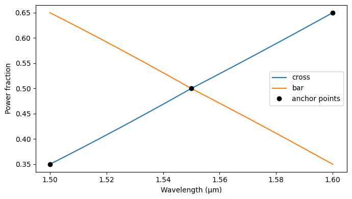
An Interpolator maps frequency to a (possibly complex) value and is evaluated at whatever frequencies the S matrix is later computed on. Below, a directional coupler receives a wavelength-dependent cross-coupling built from 3 anchor points, mimicking the wavelength sensitivity of a real coupler. The automatic bar coefficient keeps the model unitary at every frequency.

lda_anchors = np.array([1.5, 1.55, 1.6])
coupling_anchors = -1j * np.sqrt([0.35, 0.5, 0.65])
c_interpolator = pf.Interpolator(pf.C_0 / lda_anchors, coupling_anchors)

dispersive_coupler = pf.DirectionalCouplerModel(c=c_interpolator).black_box_component(
    name="dispersive_coupler"
)

lda = np.linspace(1.5, 1.6, 201)
s = dispersive_coupler.s_matrix(pf.C_0 / lda)

fig, ax = plt.subplots(1, 1, figsize=(7, 4), tight_layout=True)
ax.plot(lda, np.abs(s[("P0@0", "P3@0")]) ** 2, label="cross")
ax.plot(lda, np.abs(s[("P0@0", "P2@0")]) ** 2, label="bar")
ax.plot(lda_anchors, [0.35, 0.5, 0.65], "o", color="black", label="anchor points")
ax.set_xlabel("Wavelength (μm)")
ax.set_ylabel("Power fraction")
_ = ax.legend()

(M, N) arrays for multimode dispersion

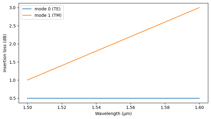
For multimode ports, a coefficient can be a 2D array of shape (M, N): one row per mode, one column per frequency. The array must match the exact frequency vector later used in the S matrix computation, so this form is best when the frequencies are known in advance, for example when loading measured or simulated data sampled on a fixed grid.

Here a 2-mode TwoPortModel gets a transmission with different loss for each mode: flat 0.5 dB for TE, and a loss ramp from 1 dB to 3 dB for TM.

loss_te_db = 0.5 * np.ones_like(lda)
loss_tm_db = 1.0 + 20.0 * (lda - 1.5)
t_modes = np.vstack([10 ** (-loss_te_db / 20), 10 ** (-loss_tm_db / 20)])
print(f"coefficient shape (M, N): {t_modes.shape}")

multimode = pf.TwoPortModel(t=t_modes).black_box_component(
    pf.virtual_port_spec(num_modes=2), name="multimode"
)
s = multimode.s_matrix(pf.C_0 / lda)

fig, ax = plt.subplots(1, 1, figsize=(7, 4), tight_layout=True)
ax.plot(lda, -20 * np.log10(np.abs(s[("P0@0", "P1@0")])), label="mode 0 (TE)")
ax.plot(lda, -20 * np.log10(np.abs(s[("P0@1", "P1@1")])), label="mode 1 (TM)")
ax.set_xlabel("Wavelength (μm)")
ax.set_ylabel("Insertion loss (dB)")
_ = ax.legend()

coefficient shape (M, N): (2, 201)

Example: black-box Mach-Zehnder interferometer

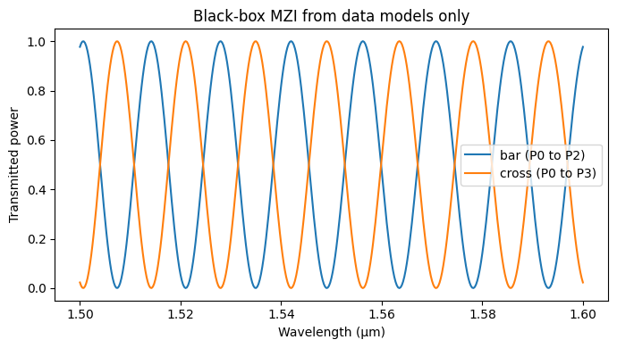
To close, a complete circuit built from data models only: two ideal 50/50 directional couplers connected by two dispersive arms of different lengths, assembled with CircuitModel. No geometry is drawn and no physical solver runs, yet the circuit produces the expected interference fringes with an FSR set by the group index and the length imbalance.

Since the components are geometry-free, all connectivity is declared with virtual connections, which inform the circuit model without requiring the ports to touch in a layout. The references only need to be spread apart so that no ports accidentally coincide (coincident ports are automatically connected by the circuit model).

def make_coupler(name):
    return pf.DirectionalCouplerModel().black_box_component(name=name)


def make_arm(name, length):
    arm_model = pf.TwoPortModel(
        propagation_length=length,
        n_eff=2.4,
        n_group=4.2,
        reference_frequency=f_ref,
    )
    return arm_model.black_box_component(name=name)


mzi = pf.Component("mzi")
splitter_ref = mzi.add_reference(make_coupler("dc_in"))
combiner_ref = mzi.add_reference(make_coupler("dc_out"))
arm_top = mzi.add_reference(make_arm("arm_top", 60.0))
arm_bottom = mzi.add_reference(make_arm("arm_bottom", 100.0))

combiner_ref.x_mid = 200
arm_top.x_mid = 100
arm_top.y_mid = 40
arm_bottom.x_mid = 100
arm_bottom.y_mid = -40

mzi.add_virtual_connection(splitter_ref, "P3", arm_top, "P0")
mzi.add_virtual_connection(splitter_ref, "P2", arm_bottom, "P0")
mzi.add_virtual_connection(arm_top, "P1", combiner_ref, "P1")
mzi.add_virtual_connection(arm_bottom, "P1", combiner_ref, "P0")

mzi.add_port(
    [splitter_ref["P0"], splitter_ref["P1"], combiner_ref["P2"], combiner_ref["P3"]]
)
mzi.add_model(pf.CircuitModel(), "Circuit")

lda = np.linspace(1.5, 1.6, 401)
s = mzi.s_matrix(pf.C_0 / lda)

fig, ax = plt.subplots(1, 1, figsize=(7, 4), tight_layout=True)
ax.plot(lda, np.abs(s[("P0@0", "P2@0")]) ** 2, label="bar (P0 to P2)")
ax.plot(lda, np.abs(s[("P0@0", "P3@0")]) ** 2, label="cross (P0 to P3)")
ax.set_xlabel("Wavelength (μm)")
ax.set_ylabel("Transmitted power")
ax.legend()
_ = ax.set_title("Black-box MZI from data models only")

Final remarks

• Pass ports=[...] explicitly whenever the sorted port names do not match the order assumed by the S matrix template.

• Use Interpolator coefficients or (M, N) arrays fitted to measured or simulated data to turn any of these into a calibrated compact model.

• Data models compose freely with solver-based models inside CircuitModel: for example, an FDTD coupler S matrix combined with WaveguideModel routing and TerminationModel on unused ports.