Noise Under Large-Signal Modulation

In this notebook, we will explore how to simulate and analyze the noise performance of an Intensity-Modulated Direct-Detection (IMDD) microwave photonic link.
While basic mathematical models often assume noise behaves as a constant, stationary background hiss, real-world large-signal modulation causes the noise to pulse alongside the signal. This is known as cyclostationary noise.
To bridge the gap between simple small-signal theory and physical reality, we will leverage PhotonForge’s abstract components to run comprehensive system-level time-domain simulations. By wiring together behavioral black-box models, such as ideal lasers, electro-optic phase shifters, and noisy photodiodes, we can easily simulate the entire link architecture and capture complex, dynamic physical effects that simple analytical formulas miss.
What You Will Learn
Link Construction: Setting up a Mach-Zehnder Modulator (MZM) based IMDD circuit using fundamental components.
Metric Extraction: Calculating signal gain (\(G_c\)), noise gain (\(G_n\)), and overall Noise Figure (NF) directly from physical time-domain waveforms.
Large-Signal Dynamics: Understanding and visualizing how a strong RF drive artificially inflates baseband noise beyond standard mathematical predictions.
Core PhotonForge Tools
pfa.cw_laser: Defines our optical carrier and Relative Intensity Noise (RIN).
pfa.phase_modulator: Provides the electro-optic effect to build our MZM.
pfa.photodiode: Converts light back to RF while injecting physical shot and thermal noise.
pfa.filter: Isolates our specific RF measurement bands.
Reference
Hosseini and A. Banai, “Noise figure of microwave photonic links operating under large-signal modulation and its application to optoelectronic oscillators,” Applied Optics 2014 53 (28), 6414–6421, doi: 10.1364/AO.53.006414
[1]:
import numpy as np
import matplotlib.pyplot as plt
from scipy.fft import rfft
import photonforge as pf
import photonforge.abstract as pfa
from photonforge.live_viewer import LiveViewer
import warnings

# Ignore the specific unconnected port warning from PhotonForge
warnings.filterwarnings(
    action='ignore',
    category=RuntimeWarning,
    module='photonforge.circuit_base'
)

viewer = LiveViewer()
LiveViewer started at http://localhost:56935
Defining Link Parameters and Physics
Before building our physical circuit, we need to define the operational parameters that govern it. We are drawing these values directly from the setup described in [1] to ensure our simulation accurately reflects their results.
This cell is broken down into four main physical domains:
Thermodynamics & RF Environment: Setting up Boltzmann’s constant (\(k_B\)), standard room temperature (\(T_0\)), and our system impedances to define the fundamental thermal noise floor, \(N_{in} = k_B T_0 B\).
Modulator (MZM) Specs: The paper specifies a half-wave voltage \(V_\pi = 3.1\) V and a photonic voltage parameter \(V_{ph} = 3.12\) V. Because PhotonForge simulates physical waveguides rather than mathematical black boxes, we map these target voltages to actual waveguide properties (effective index, length) and calculate the exact DC bias voltage (\(V_b\)) required to hold the physical structure precisely at quadrature (\(\Gamma_0 = \pi/2\)).
Optoelectronics (Laser & PD): We define an ideal photodiode responsivity (\(\rho = 1.0\) A/W) and use the \(V_{ph}\) equation to back-calculate the exact continuous-wave (CW) laser power (\(P_0\)) needed to drive the system. We also convert the laser’s Relative Intensity Noise (RIN) from logarithmic units (dB/Hz) to linear units (1/Hz) for the analytical formulas.
Simulation Bands: We choose an RF tone of 100 MHz and a wide observation bandwidth of 20 MHz.
[2]:
# 1. Thermodynamics & System Environment
kB = 1.380649e-23
T0 = 290.0
RL = 50.0 # ohm (Load resistor)
Z0 = 50.0 # ohm (Electrical port impedance used for wave <-> voltage conversion)

# 2. Modulator (MZM) Specifications
Vpi = 3.1 # V (Voltage required for a pi phase shift)
Vph = 3.12 # V (Photonic voltage parameter from the paper)
Gamma0 = np.pi / 2 # Quadrature bias point target

# Physical waveguide properties for the MZM phase shifter
lambda0 = 1.55 # um (Optical carrier wavelength)
ps_n_eff = 2.4 # Effective index of the waveguide
ps_length_um = 1.0 # Arbitrary length for the phase shifter
ps_v_piL = Vpi * ps_length_um # Vpi*L product

# Calculate the exact DC bias voltage (Vb) needed to achieve quadrature.
# A physical MZM has a static phase difference due to its optical path length;
# we offset this static phase (phi0) to land exactly at pi/2.
m = int(2 * ps_n_eff * ps_length_um / lambda0)
phi0 = 2 * np.pi * ps_n_eff * ps_length_um / lambda0
Vb = (ps_v_piL / (np.pi * ps_length_um)) * ((np.pi / 2 + m * np.pi) - phi0)

# 3. Optoelectronics: Laser & Photodiode
rho = 1.0 # A/W (Photodiode responsivity)
TIA_gain = RL # V/A (Transimpedance amplifier gain equivalent to RL)
alpha_ins = 1.0 # MZM insertion loss (linear, 1.0 = lossless)

# Back-calculate required laser power using the paper's Vph relationship:
# Vph = alpha_ins * P0 * rho * RL / 2
P0_laser = 2 * Vph / (alpha_ins * rho * TIA_gain) # W
Id_avg = Vph / RL # A (Average DC photocurrent at quadrature)

# Convert RIN from logarithmic specification to linear
RIN_dB_per_Hz = -165.0
RIN = 10**(RIN_dB_per_Hz / 10) # linear 1/Hz

# 4. Simulation Measurement Bands
f_rf = 100e6 # 100 MHz RF drive tone
B = 20e6     # 20 MHz measurement bandwidth

# Calculate available input thermal noise power (Nin) for NF definitions
Nin = kB * T0 * B

# Print out sanity checks for the derived values
print('P0_laser (W):', P0_laser)
print('Id_avg (mA):', Id_avg * 1e3)
print('RIN (1/Hz):', RIN)
print('Nin (dBm):', 10 * np.log10(Nin / 1e-3))
P0_laser (W): 0.12480000000000001
Id_avg (mA): 62.400000000000006
RIN (1/Hz): 3.1622776601683796e-17
Nin (dBm): -100.9648872375883
Unlike analytical equations that directly spit out a “Noise Figure,” a time-domain simulation outputs raw, physical waveforms - just like an oscilloscope. To extract meaningful performance metrics like signal gain and noise power, we need to act as a virtual spectrum analyzer.
This cell defines a suite of DSP utility functions to process our simulated voltage arrays:
Tone Extraction (
fit_single_tone): To measure the signal power, we need to isolate the fundamental RF tone from the noisy waveform. We use orthogonal projection to find the Fourier coefficients (\(a\) and \(b\)) for our target frequency \(f_0\):\[v(t) \approx a \cos(2\pi f_0 t) + b \sin(2\pi f_0 t)\]From these coefficients, we can calculate the peak amplitude and phase of the signal.
RF Power Calculation (
power_of_tone): Converts a peak voltage amplitude into average electrical power (Watts) across our system’s load impedance (\(R_L\)).
[3]:
from dataclasses import dataclass
from scipy import signal

@dataclass
class ToneFit:
    a_cos: float
    b_sin: float
    amp_peak: float
    phase_rad: float

def fit_single_tone(v: np.ndarray, t: np.ndarray, f0: float) -> ToneFit:
    """Least-squares fit v(t) ≈ a cos(2πf0 t) + b sin(2πf0 t)."""
    w = 2 * np.pi * f0
    c = np.cos(w * t)
    s = np.sin(w * t)

    # Orthogonal projection (works well when many cycles are present)
    a = 2.0 * np.mean(v * c)
    b = 2.0 * np.mean(v * s)

    amp = np.sqrt(a * a + b * b)
    phase = np.arctan2(-b, a)  # so that amp*cos(wt+phase)
    return ToneFit(a_cos=a, b_sin=b, amp_peak=amp, phase_rad=phase)

def power_of_tone(amp_peak: float, R: float) -> float:
    return (amp_peak * amp_peak) / (2 * R)
Calculating Equivalent Noise Bandwidth
When dealing with noise in any physical or simulated system, the shape of your measurement filter matters. A real-world bandpass filter does not have perfectly sharp “brick-wall” edges; it has roll-off.
To accurately compare our simulated noise to theoretical formulas, we must calculate the Equivalent Noise Bandwidth (ENBW) of our digital filter. The ENBW is the width of an ideal, perfectly rectangular filter that would pass the exact same amount of white noise power as our actual filter.
The mathematical definition is:
where \(H(f)\) is the frequency response of the filter.
[4]:
def calculate_enbw(bpf, fs):
    """
    Calculates the exact Equivalent Noise Bandwidth of a pre-existing PhotonForge filter component.
    """
    time_step = 1.0 / fs
    steps = 200000

    # Inject a discrete impulse
    ts = bpf.setup_time_stepper(time_step=time_step, carrier_frequency=193e12)
    ts.reset()

    impulse_arr = np.zeros(steps)
    impulse_arr[0] = 1.0  # The impulse

    # Map the impulse to the input port
    in_port_name = "E0@0"
    out_port_name = "E1@0"
    inputs = pf.TimeSeries({in_port_name:impulse_arr}, time_step)

    outputs = ts.step(inputs, show_progress=False)

    # Extract the impulse response and calculate the Power Transfer Function
    h = np.real(outputs[out_port_name])
    H = rfft(h)
    H_power = np.abs(H)**2

    # ENBW is the integral of the power response divided by the peak
    df = fs / steps
    enbw_hz = np.sum(H_power) * df / np.max(H_power)

    return float(enbw_hz)
Before wiring up the main optical circuit, we must establish the underlying simulation environment and define our custom electrical filters.
Technology & Ports: We initialize PhotonForge’s base technology and set up “virtual ports.” These act as the standardized optical and electrical interfaces connecting our components.
RF Bandpass Filter (BPF): Created with
pfa.filter(shape="bp", ...), this filter isolates our 100 MHz signal and the surrounding 20 MHz noise band, throwing away out-of-band noise to allow for clean metric extraction.Input Low-Pass Filter (LPF): Created with
pfa.filter(shape="lp", ...), this scrubs high-frequency wideband noise from the input RF drive while perfectly preserving our crucial DC bias voltage.
[5]:
# Technology
pf.config.default_technology = pf.basic_technology()

# Create a highly selective, lossless rectangular bandpass filter
bpf = pfa.filter(
    family="rectangular",
    shape="bp",
    f_cutoff=(f_rf - B / 2, f_rf + B / 2),
    taps=4001,
    insertion_loss=0.0,
)

# Create an Input Low-Pass Filter to scrub high-frequency noise but preserve DC Bias
in_filter = pfa.filter(
    family="rectangular",
    shape="lp",
    f_cutoff=f_rf + B,
    taps=4001,
    insertion_loss=0.0,
)
Building the Core IMDD Link
This cell is the heart of our physical simulation. Here, we define a function build_imdd_link that dynamically generates our entire IMDD circuit based on the sweep parameters (like RF power and noise inclusion flags).
We construct the system component by component:
The Mach-Zehnder Modulator (MZM): Built using
pfa.directional_coupler()for ideal 50/50 splitting andpfa.phase_modulator(...)as the EO phase shifter, which bundles the frequency-domain model and time-domain drive law into a single component.The RF Drive Source: Created with
pfa.signal_source(...), it physically models the electrical drive by combining the DC bias (\(V_b\)) to hold the MZM at quadrature, the large-signal RF tone (\(V_{sig}\)), and the fundamental input thermal noise limit defined by \(k_B T_0\).The CW Laser: Created with
pfa.cw_laser(...), it is the optical power house of the link. It can dynamically toggle Relative Intensity Noise (RIN) on or off, allowing us to isolate and study different noise contributors independently.The Photodiode (PD): Created with
pfa.photodiode(...), it converts the modulated light back into an electrical signal while incorporating receiver thermal noise (toggled viainclude_thermal).
Note: PhotonForge uses traveling wave amplitudes rather than raw voltages for its electrical ports. You will notice we divide our calculated peak voltages by :math:`sqrt{Z_0}` to properly format them for the ``pfa.signal_source``.
[6]:
def build_imdd_link(
    *,
    f_opt: float,
    f_rf: float,
    B: float,
    Pin_W: float,
    include_rin: bool,
    include_thermal: bool,
    seed: int,
):
    """Build IMDD link (laser -> MZM -> photodiode -> RF BPF)."""

    # Optical couplers
    directional_coupler = pfa.directional_coupler()

    # EO phase shifter tuned so that V_pi ≈ Vpi for the chosen length
    length_um = 1.0
    v_piL = Vpi * length_um

    phase_shifter = pfa.phase_modulator(
        n_eff=2.4,
        n_group=4.0,
        length=length_um,
        v_piL=v_piL,
        z0=Z0,
        propagation_loss=0.0,
    )

    # Electrical drive: V(t) = Vb + Vsig*cos(2πf_rf t) + n(t)
    Vsig = np.sqrt(2 * Pin_W * RL)
    amp_wave = Vsig / np.sqrt(Z0)  # equals sqrt(2*Pin_W)
    off_wave = Vb / np.sqrt(Z0)

    # Input thermal noise (available power kBTB). signal_source uses a one-sided ASD in sqrt(W/Hz).
    noise_asd = np.sqrt(kB * T0)

    rf_source = pfa.signal_source(
        frequency=f_rf,
        amplitude=amp_wave,
        offset=off_wave,
        waveform="sine",
        noise=noise_asd,
        seed=seed,
    )

    # Laser
    laser = pfa.cw_laser(
        power=P0_laser,
        rel_intensity_noise=(RIN if include_rin else 0.0),
        linewidth=0.0,
        seed=seed + 1,
    )

    laser_dark = pfa.cw_laser(power=0.0)

    # Photodiode + TIA
    thermal_noise_psd = (4 * kB * T0 / RL) if include_thermal else 0.0  # A^2/Hz (approx)
    pd = pfa.photodiode(
        responsivity=rho,
        gain=TIA_gain,
        thermal_noise=thermal_noise_psd,
        z0=Z0,
        seed=seed + 2,
    )

    # Assemble netlist
    netlist = {
        "name": "IMDD_Link_LargeSignalNF",
        "instances": {
            "in_dc": {"component": directional_coupler, "origin": (0.0, 0.0)},
            "out_dc": {"component": directional_coupler, "origin": (9.0, 0.0)},
            "ps": {"component": phase_shifter, "origin": (7.0, 1.0)},
            "rf": {"component": rf_source},
            "laser": {"component": laser, "origin": (-3.0, 0.8)},
            "dark": {"component": laser_dark, "origin": (-3.0, -0.8)},
            "pd": {"component": pd, "origin": (12.0, 1.0)},
            "bpf_in": {"component": in_filter, "origin": (12.0, -0.2)},
            "bpf_out": {"component": bpf, "origin": (12.0, -0.2)},
        },
        "connections": [
            # Optical inputs
            (("laser", "P0"), ("in_dc", "P1")),
            (("dark", "P0"), ("in_dc", "P0")),
            # MZM arm
            (("ps", "P0"), ("in_dc", "P3")),
            (("out_dc", "P1"), ("ps", "P1")),
            # Electrical drive
            (("bpf_in", "E1"), ("ps", "E0")),
            (("rf", "E0"), ("bpf_in", "E0")),
            # Optical to photodiode (pick one MZM output)
            (("pd", "P0"), ("out_dc", "P2")),
            # # Electrical chain: PD -> BPF
            (("bpf_out", "E0"), ("pd", "E0")),
        ],
        "virtual connections": [
            (("in_dc", "P2"), ("out_dc", "P0")),
        ],
        # Expose the BPF output
        "ports": [("bpf_out", "E1")],
        "models": [(pf.CircuitModel(), "Circuit")],
    }

    top = pf.component_from_netlist(netlist)
    viewer(top)
    # Reference indices (match insertion order of instances)
    instance_names = list(netlist["instances"].keys())
    ref_indices = {
        "rf_drive": instance_names.index("bpf_in"),
        "out_dc": instance_names.index("out_dc"),
    }

    return top, ref_indices
Executing the Time-Domain Simulation
With our physical parameters and circuit layout defined, we need a way to easily run the simulation across different RF power levels. This cell defines run_link_once, an execution wrapper that dynamically builds the link and runs the time-stepping engine for a single set of conditions.
Here is what happens under the hood during execution:
Circuit Instantiation: It calls our
build_imdd_linkfunction to construct a fresh circuit tailored to the current RF input power and noise settings.Placing Probes (Monitors): Just like hooking up an oscilloscope in the lab, we place specific monitors in the circuit. We tap into the RF input drive and the optical signal right before it hits the photodiode. (The final RF output is automatically monitored because we exposed it as a main circuit port).
Simulation Engine: We initialize PhotonForge’s
time_stepper, defining the central optical carrier frequency (\(f_{opt}\)) and the frequency span to track. We then step the simulation forward in time.Data Formatting: PhotonForge natively tracks electrical signals as traveling wave amplitudes to accurately model physical power flow. Before returning the data, we convert these wave amplitudes back into standard absolute voltages using the relationship \(V = A_{wave} \sqrt{Z_0}\).
[7]:
def run_link_once(
    *,
    Pin_dBm: float,
    include_rin: bool,
    include_thermal: bool,
    seed: int,
    time_step: float,
    steps: int,
):
    Pin_W = 1e-3 * 10 ** (Pin_dBm / 10)
    f_opt = pf.C_0 / 1.55

    link, ref_indices = build_imdd_link(
        f_opt=f_opt,
        f_rf=f_rf,
        B=B,
        Pin_W=Pin_W,
        include_rin=include_rin,
        include_thermal=include_thermal,
        seed=seed,
    )

    # locate references for monitors (by instance insertion order)
    rf_ref = link.references[ref_indices["rf_drive"]]
    outdc_ref = link.references[ref_indices["out_dc"]]

    # setup and run
    freq_span = 2e9
    frequencies = np.linspace(f_opt - freq_span, f_opt + freq_span, 101)

    ts = link.setup_time_stepper(
        time_step=time_step,
        carrier_frequency=f_opt,
        time_stepper_kwargs={
            "frequencies": frequencies,
            "monitors": {
                "rf_drive": rf_ref["E1"],
                # Optical monitor just before PD (output directional coupler port feeding PD)
                "opt_pre_pd": outdc_ref["P2"],
            },
        },
    )

    out = ts.step(steps=steps, time_step=time_step)

    t = out.times

    drive_wave = np.real(out["rf_drive@0+"])
    vout_wave = np.real(out["E0@0"])  # exposed port: (bpf, E1)

    # Optical field monitor (complex envelope)
    Aopt_pre_pd = out["opt_pre_pd@0+"]

    v_in = drive_wave * np.sqrt(Z0)
    v_out = vout_wave * np.sqrt(Z0)

    return t, v_in, v_out, Aopt_pre_pd
Metric Extraction from Waveforms
This section processes our raw time-domain waveforms to compute Signal Gain (\(G_c\)), Noise Gain (\(G_n\)), and Noise Figure (NF).
Because we are working with raw signal arrays containing both the powerful RF tone and the microscopic noise fluctuations, we must carefully separate them:
Tone Stripping: For each measurement point, we fit an ideal sine wave to the fundamental RF carrier (\(100\) MHz) and subtract it from the raw waveform. What remains is pure residual noise.
Band-limited Noise Power:
For the Output Noise (:math:`N_{out}`): Because our simulated circuit already includes a highly selective physical brick-wall Bandpass Filter (BPF), all out-of-band noise is gone. We can instantly find the in-band noise power simply by taking the statistical variance of the residual waveform (
np.var() / R).For the Input/Modulator Noise (:math:`N_{in}` and :math:`G_n`): We use a
scipy.signal.periodogramto calculate the Power Spectral Density (PSD) and numerically integrate it exactly over our \(20\) MHz observation window.
Isolating :math:`G_n`: To find the noise gain strictly from the modulator (without the photodiode’s thermal/shot noise), we tap into the optical monitor just before the PD, mathematically convert its complex envelope into an ideal equivalent voltage, and measure its noise power.
[8]:
def brickwall_band_power_W(v: np.ndarray, fs: float, f_lo: float, f_hi: float, R: float) -> float:
    """Calculates noise power (W) inside a strict [f_lo, f_hi] frequency band
    by integrating a one-sided periodogram (PSD)."""
    # Remove DC offset
    v = v - np.mean(v)

    # Calculate Power Spectral Density (V^2/Hz)
    f, Pxx = signal.periodogram(
        v, fs=fs, window="boxcar", detrend="constant",
        scaling="density", return_onesided=True,
    )

    # Create a boolean mask to isolate our exact frequency band
    m = (f >= f_lo) & (f <= f_hi)
    if not np.any(m):
        return 0.0

    # Numerically integrate the PSD over the band and convert to Watts
    v2 = float(np.trapezoid(Pxx[m], f[m]))
    return v2 / R

def measure_Gc_Gn_NF_photonforge(*, t: np.ndarray, v_in: np.ndarray, v_out: np.ndarray,
                                 Aopt_pre_pd: np.ndarray, Pin_W_cmd: float,
                                 steady_state: bool = True) -> dict:
    """Extracts Gc, Gn, and NF directly from PhotonForge time-domain waveforms."""

    # Drop initial simulation transients to ensure we only measure steady-state
    drop = 10000 if steady_state else 0
    tt = t[drop:]
    vin = v_in[drop:]
    vout = v_out[drop:]
    fs = 1.0 / (t[1] - t[0])
    f_lo, f_hi = f_rf - B / 2, f_rf + B / 2

    # Remove DC bias from the waveforms
    vin_ac = vin - np.mean(vin)
    vout_ac = vout - np.mean(vout)

    # 1. Extract the signal tones
    fit_in = fit_single_tone(vin_ac, tt, f_rf)
    fit_out = fit_single_tone(vout_ac, tt, f_rf)
    Pin_W_meas = power_of_tone(fit_in.amp_peak, RL)
    Pout_sig_W = power_of_tone(fit_out.amp_peak, RL)

    # 2. Strip the fundamental RF tones to leave only the residual noise
    vin_res = vin_ac - (fit_in.a_cos * np.cos(2 * np.pi * f_rf * tt) + fit_in.b_sin * np.sin(2 * np.pi * f_rf * tt))
    vout_res = vout_ac - (fit_out.a_cos * np.cos(2 * np.pi * f_rf * tt) + fit_out.b_sin * np.sin(2 * np.pi * f_rf * tt))

    # Calculate input noise power via periodogram integration
    Nin_W_meas = brickwall_band_power_W(vin_res, fs, f_lo, f_hi, RL)

    # Since v_out already passed through our physical brick-wall BPF in the simulation,
    # we can bypass the periodogram and calculate total in-band noise power directly via variance!
    Nout_W_meas = float(np.var(vout_res)) / RL

    # Calculate Signal Gain (Gc) and true physical Noise Figure (NF)
    Gc = Pout_sig_W / (Pin_W_cmd + 1e-300)
    NF_meas = (Pin_W_meas / (Nin_W_meas + 1e-300)) / (Pout_sig_W / (Nout_W_meas + 1e-300))

    # 3. Calculate Modulator Noise Gain (Gn)
    # Convert pre-PD optical envelope to an ideal equivalent voltage
    v_mod = rho * (np.abs(Aopt_pre_pd) ** 2) * TIA_gain
    vmod = v_mod[drop:]
    vmod_ac = vmod - np.mean(vmod)

    # Strip the tone and measure the modulator's specific noise contribution
    fit_mod = fit_single_tone(vmod_ac, tt, f_rf)
    vmod_res = vmod_ac - (fit_mod.a_cos * np.cos(2 * np.pi * f_rf * tt) + fit_mod.b_sin * np.sin(2 * np.pi * f_rf * tt))

    Nout_mod_W = brickwall_band_power_W(vmod_res, fs, f_lo, f_hi, RL)
    Gn_mod_meas = Nout_mod_W / (Nin_W_meas + 1e-300)

    # Return only the essential metrics needed for plotting
    return {
        "Pin_W_meas": float(Pin_W_meas),
        "Gc": float(Gc),
        "Gn_mod_meas": float(Gn_mod_meas),
        "NF_meas": float(NF_meas),
    }
Noise and Signal Gain Measurement
With our measurement functions in place, we are ready to run the core simulation sweep. We will iterate over a range of RF input powers from \(-20\) dBm to \(+15\) dBm. This sweep allows us to observe how the link transitions from a linear, small-signal regime into nonlinear, large-signal operation.
Key Simulation Parameters:
Sampling Rate (:math:`f_s`): We set the sampling frequency to 40 times the RF carrier frequency. This heavy oversampling is crucial to prevent aliasing and accurately capture the high-frequency harmonics generated during large-signal modulation.
Duration: We run each power level for 20,000 time steps. Noise is inherently random, so we need a sufficiently long time record for our statistical periodogram to yield a stable, accurate measurement of the average noise power. Increase this number for more accurate results.
Isolating Noise Sources: Notice that we set
include_rin=Falsein this specific loop. By turning off the laser’s Relative Intensity Noise, we isolate the baseline thermal and shot noise behaviors. We will run a separate sweep later with RIN enabled to see its massive cyclostationary impact!
[9]:
# Sweep RF input power from -20 dBm to +15 dBm in 5 dB increments
Pin_dBm_sweep = np.arange(-20.0, 20.0, 5.0)

steps = 20000
seed0 = 100

# Set a high sampling frequency (40x the RF tone) to capture harmonics and noise
fs = 40 * f_rf
time_step = 1 / fs

# Initialize lists to store the extracted metrics for each power level
Gc_dB = []
Gn_mod_meas_dB = []

for i, Pin_dBm in enumerate(Pin_dBm_sweep):
    # Convert commanded dBm to linear Watts for the gain calculations
    Pin_W_cmd = 1e-3 * 10**(Pin_dBm / 10)

    # Run the physical simulation for this specific power level.
    # Note: RIN is explicitly turned OFF here to establish a thermal/shot noise baseline.
    t, v_in, v_out, Aopt_pre_pd = run_link_once(
        Pin_dBm=float(Pin_dBm),
        include_rin=False,
        include_thermal=True,
        seed=seed0 + i,
        time_step=time_step,
        steps=steps,
    )

    # Pass the raw waveforms to our DSP function to extract the metrics
    m = measure_Gc_Gn_NF_photonforge(
        t=t,
        v_in=v_in,
        v_out=v_out,
        Aopt_pre_pd=Aopt_pre_pd,
        Pin_W_cmd=Pin_W_cmd,
        steady_state=True,
    )

    # Convert the linear power and gain ratios back into decibels (dB / dBm)
    # A tiny offset (1e-300) is added to prevent log10(0) errors if a value drops to zero
    Gc_dB.append(10 * np.log10(m['Gc'] + 1e-300))
    Gn_mod_meas_dB.append(10 * np.log10(m['Gn_mod_meas'] + 1e-300))
[10]:
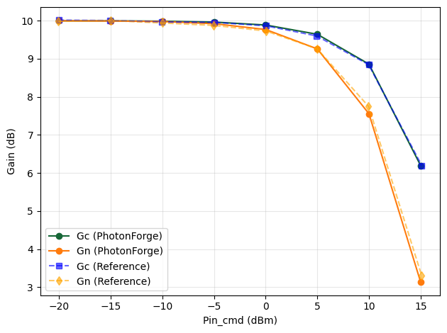
# Reference data (Gc)
pin_gc_ref = [-20.04236, -15.06066, -10.07911, -4.96967, 0.01160, 4.94935, 9.96967, 15.10764]
gc_ref = [10.01362, 10.00399, 9.96728, 9.95740, 9.86655, 9.59981, 8.84560, 6.19607]

# Reference data (Gn)
pin_gn_ref = [-20.04251, -15.01808, -9.99409, -5.01268, 0.01088, 4.99013, 9.96383, 15.09229]
gn_ref = [9.98655, 10.00390, 9.94004, 9.87626, 9.73119, 9.26132, 7.74916, 3.31285]

plt.figure()

# Current simulation plots
plt.plot(Pin_dBm_sweep, Gc_dB, 'o-', label='Gc (PhotonForge)')
plt.plot(Pin_dBm_sweep, Gn_mod_meas_dB, 'o-', label='Gn (PhotonForge)')

# Reference data plots
plt.plot(pin_gc_ref, gc_ref, 's--', color='blue', alpha=0.6, label='Gc (Reference)')
plt.plot(pin_gn_ref, gn_ref, 'd--', color='orange', alpha=0.6, label='Gn (Reference)')

plt.xlabel('Pin_cmd (dBm)')
plt.ylabel('Gain (dB)')
plt.grid(True, alpha=0.3)
plt.legend()
plt.tight_layout()
plt.show()
The Cyclostationary Sweep (Enabling RIN)
Now for the main event. We run the exact same power sweep, but with two critical changes:
``include_rin = True``: We turn the laser’s Relative Intensity Noise back on. Because RIN scales with the square of the instantaneous optical power, the large RF swings will cause the noise to fold and multiply, creating the cyclostationary effect.
``steps = 200000``: Notice we increased the simulation duration by a factor of 10. Cyclostationary noise is highly statistical and dynamic. To get a clean, converged measurement of the total Noise Figure (NF), we must observe the system over a much longer time window.
[11]:
# Increase time steps tenfold to allow statistical noise variance to fully converge
steps = 200000

# Re-initialize arrays specifically for the total Noise Figure extraction
NF_meas_dB = []
Pin_meas_dBm = []

for i, Pin_dBm in enumerate(Pin_dBm_sweep):
    Pin_W_cmd = 1e-3 * 10 ** (Pin_dBm / 10)

    # Run the physical simulation.
    # CRITICAL CHANGE: include_rin is now True!
    t, v_in, v_out, Aopt_pre_pd = run_link_once(
        Pin_dBm=float(Pin_dBm),
        include_rin=True,
        include_thermal=True,
        seed=seed0 + i,
        time_step=time_step,
        steps=steps,
    )

    # Extract the metrics from the long-duration waveforms
    m = measure_Gc_Gn_NF_photonforge(
        t=t,
        v_in=v_in,
        v_out=v_out,
        Aopt_pre_pd=Aopt_pre_pd,
        Pin_W_cmd=Pin_W_cmd,
        steady_state=True,
    )

    # Store the measured Total Noise Figure and actual measured Input Power
    NF_meas_dB.append(10 * np.log10(m['NF_meas'] + 1e-300))
    Pin_meas_dBm.append(10 * np.log10(m['Pin_W_meas'] / 1e-3 + 1e-300))
Stationary vs. Cyclostationary Noise
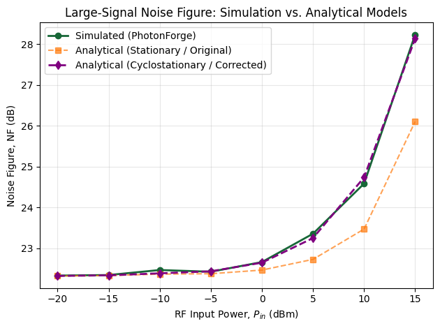
When comparing our time-domain simulation to the paper’s standard analytical formula, you will notice a growing divergence at high RF input powers (large-signal regime). The simulated Noise Figure (NF) climbs systematically higher than the mathematical prediction.
This mismatch is not a simulation error; rather, it highlights a physical limitation of the standard analytical formula:
The Stationary Assumption (Standard Formula): The paper’s baseline formula relies on a small-signal approximation:
\[NF = 10 \log_{10} \left[ \frac{2G_n(P_{in})}{G_c(P_{in})} + \frac{1}{G_c(P_{in})} + \frac{\langle I_D \rangle^2 N_{rin} R_L + 2e\langle I_D \rangle R_L}{G_c(P_{in}) k_B T_0} \right]\]It assumes that Shot noise and Relative Intensity Noise (RIN) act as a constant background hiss dictated strictly by the time-averaged DC photocurrent (\(\langle I_D \rangle\)).
The Cyclostationary Reality: Under large-signal RF drive, the MZM optical output swings violently, causing the noise itself to pulse at the RF carrier frequency. Because RIN power is proportional to the square of the instantaneous current (\(I_D(t)^2\)), its true time-averaged power grows faster than the simple DC average predicts.
The Correction Factor: By applying a cyclostationary correction factor - specifically, scaling the RIN term by \(1.5 - 0.5 J_0(2m)\), where \(m\) is the modulation index - we can mathematically capture this large-signal noise inflation.
The figure below displays all three curves to demonstrate how the cyclostationary correction perfectly bridges the gap between the paper’s original math and the physical simulation.
[12]:
import scipy.special as sp
from scipy.constants import e

# 1. Standard Analytical Calculation (Stationary)
# Convert Gain from dB to Linear
gc_lin = 10 ** (np.array(gc_ref) / 10)
gn_lin = 10 ** (np.array(gn_ref) / 10)

# Calculate Theoretical Noise Figure Terms
term1 = 2 * (gn_lin / gc_lin)
term2 = 1 / gc_lin

thermal_noise_base = kB * T0
shot_noise = 2 * e * Id_avg * RL
rin_noise = (Id_avg ** 2) * RIN * RL

term3 = (rin_noise + shot_noise) / (gc_lin * thermal_noise_base)

# Total Noise Factor (Stationary)
enbw = calculate_enbw(bpf, fs)
F_linear = term1 + term2 + term3 * enbw / B
nf_calculated_dB = 10 * np.log10(F_linear)

# 2. Corrected Analytical Calculation (Cyclostationary)
# Calculate Peak RF Voltage and Modulation Index (m)
V_peak = np.sqrt(2 * RL * (1e-3 * 10**(Pin_dBm_sweep / 10)))
m_mod = np.pi * V_peak / Vpi

# Calculate Cyclostationary RIN Enhancement Factor
rin_enhancement = 1.5 - 0.5 * sp.j0(2 * m_mod)

# Apply to the Noise Terms (Shot noise remains unchanged)
rin_noise_cyclo = (Id_avg ** 2) * rin_enhancement * RIN * RL

# Total Noise Factor (Cyclostationary)
term3_cyclo = (rin_noise_cyclo + shot_noise) / (gc_lin * thermal_noise_base)
F_linear_cyclo = term1 + term2 + term3_cyclo * enbw / B
nf_calculated_cyclo_dB = 10 * np.log10(F_linear_cyclo)

# 3. Final Unified Plot
plt.figure()

# Simulated
plt.plot(Pin_dBm_sweep, NF_meas_dB, 'o-', linewidth=2, label='Simulated (PhotonForge)')

# Analytical Models
plt.plot(Pin_dBm_sweep, nf_calculated_dB, 's--', alpha=0.7, label='Analytical (Stationary / Original)')
plt.plot(Pin_dBm_sweep, nf_calculated_cyclo_dB, 'd--', color='purple', linewidth=2, label='Analytical (Cyclostationary / Corrected)')

plt.xlabel('RF Input Power, $P_{in}$ (dBm)')
plt.ylabel('Noise Figure, NF (dB)')
plt.title('Large-Signal Noise Figure: Simulation vs. Analytical Models')
plt.grid(True, alpha=0.3)
plt.legend()
plt.tight_layout()
plt.show()