Time-Domain Simulation of a Mach–Zehnder Interferometer

In this notebook, we design and simulate a passive Mach–Zehnder Interferometer (MZI) in the time domain. This structure contains no active modulation components—all elements are passive, including the spiral delay line used to introduce an optical path length difference between the two arms.

The goal is to demonstrate how PhotonForge can perform layout-aware time-domain simulations of passive photonic circuits with minimal user effort.

By simply calling the time-stepper once on the assembled MZI, PhotonForge automatically:

1. Computes the frequency-domain S‑matrix of each component (using analytical models or full-wave solvers like Tidy3D).

2. Generates a pole–residue fit for each response to enable efficient time-domain evaluation.

3. Propagates the input waveforms through the circuit to obtain the output signals.

This workflow requires no manual fitting or convolution code—PhotonForge handles the entire process internally.

import numpy as np
import photonforge as pf
import siepic_forge as siepic_pdk
from matplotlib import pyplot as plt

We begin by setting up the default technology, component parameters and frequencies for our MZI simulation.

# Set the default technology to SiEPIC OpenEBL
pf.config.default_technology = siepic_pdk.ebeam()

# Define default keyword arguments for all components
pf.config.default_kwargs = {
    "radius": 5,  # default bend radius in microns
    "euler_fraction": 0.5,  # fraction of bend length as Euler curve
    "port_spec": "TE_1550_500",  # default port specification (waveguide type)
}

# Define the optical carrier frequency (around 1550 nm wavelength)
f_c = 193.4e12  # Hz

# Define the electrical modulation frequency
f_m = 10e9  # Hz

Directional Coupler

We create a directional coupler using an S-bend geometry with specified coupling distance, length, and offset parameters, designed for 50% coupling efficiency at 1550 nm wavelength. We also add the analytical built-in DirectionalCouplerModel model for the coupler to enable efficient circuit-level simulations without full-field computation.

# Create a parametric S-bend directional coupler
directional_coupler = pf.parametric.s_bend_coupler(
    coupling_distance=0.6,  # gap between coupling waveguides (µm)
    coupling_length=4.7,  # length of coupling region (µm)
    s_bend_length=5,  # length of S-bend transition (µm)
    s_bend_offset=1,  # lateral offset of S-bend (µm)
)

# Define symmetry relations for Tidy3D simulation
directional_coupler.models["Tidy3D"].port_symmetries = [
    ("P1", "P0", "P3", "P2"),  # reflection across x-axis
    ("P2", "P3", "P0", "P1"),  # reflection across y-axis
    ("P3", "P2", "P1", "P0"),  # inversion symmetry
]

# Add analytical model for faster circuit simulations
directional_coupler.add_model(pf.DirectionalCouplerModel(), "Analytical Model")

# Display the coupler
directional_coupler

Then, we define a rectangular spiral with 7 turns, aligned along the y-axis:

spiral = pf.parametric.rectangular_spiral(turns=7, align_ports="y")
spiral

and a straight waveguide to match the spiral length minus the modulator length.

wg = pf.parametric.straight(length=spiral.size()[0])
wg

MZI Assembly

We now integrate the previously defined components to construct the full MZI. External ports are collected from the two couplers and the modulator’s electrical control port, making it possible to inject optical signals and apply modulation voltage. A CircuitModel is added so that PhotonForge can simulate the device as a network of interconnected subcomponents in the time domain. This completes the layout and connectivity for our MZI, ready for time-domain simulation with optical and electrical inputs.

# Define netlist for assembling the tunable photonic unit
netlist_mzi = {
    "name": "MZI",
    "instances": {
        "dc0": directional_coupler,  # input coupler
        "spiral": spiral,
        "wg": wg,
        "dc1": directional_coupler,  # output coupler
    },
    # Explicitly define connections between component ports
    "connections": [
        (("wg", "P0"), ("dc0", "P2")),
        (("dc1", "P0"), ("wg", "P1")),
        (("spiral", "P0"), ("dc0", "P3")),
    ],
    # Define external ports of the tunable unit
    "ports": [("dc0", "P0"), ("dc0", "P1"), ("dc1", "P2"), ("dc1", "P3")],
    # Assign circuit model to the assembled unit
    "models": [(pf.CircuitModel(), "Circuit")],
}

# Create a photonic component from the defined netlist
mzi = pf.component_from_netlist(netlist_mzi)

# Visualize the assembled tunable unit
mzi

Time-Stepper Initialization

One of the key advantages of PhotonForge is how simple it is for the user to set up a time-domain simulation. With just a few lines of code to create a TimeStepper, PhotonForge magically handles all the complexity behind the scenes:

• It computes the frequency-domain S‑matrix for each component in the MZI.

• It automatically generates a pole–residue fit of these responses.

• It prepares the time-domain solver that will propagate the input waveforms through the MZI.

The user only needs to provide:

• The desired time_step

• The optical carrier_frequency

• A frequency sweep range for spectral fitting

Once this is done, the simulation engine is fully initialized and ready to evolve the optical fields through the MZI over time—no manual fitting, no extra setup.

# Choose a time step small enough to resolve the modulation period
time_step = 0.001 / f_m

# Create a time-stepper for the MZI with the given simulation parameters
ts = mzi.setup_time_stepper(
    time_step=time_step,
    carrier_frequency=f_c,
    time_stepper_kwargs={
        "frequencies": np.linspace(f_c - 200 * f_m, f_c + 200 * f_m, 100)
    },
)

Loading cached simulation from .tidy3d/pf_cache/L3M/ms_info-EOPN3HGFTNAF45CHOW5APKKAFTV5TCO2IR2SEA5377VZ56EHVNEQ.json.
Loading cached simulation from .tidy3d/pf_cache/B75/ms_info-ZTMMYLSH4WJGHIKDBL6ULUW5TEEXX5UKS6ZTSAD42TZMUYN6SXPA.json.
Loading cached simulation from .tidy3d/pf_cache/G64/ms_info-6REAIQY4P6UMVBAHGL7J3NIHZLLP3Y6GGNTIKZITE2S252KEDYEQ.json.
Loading cached simulation from .tidy3d/pf_cache/CUE/ms_info-C7O4VGXYTVXJFSPY3FG7EJSSQL3AETANHXD4FUQIXJUSIQEYWDIQ.json.
Progress: 100%

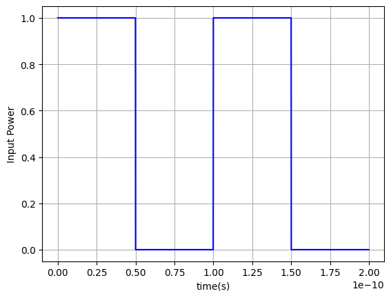
Input Signal Definition

We define the electrical and optical signals that drive the MZI during the time-domain simulation. These inputs will be used by the time-stepper to propagate signals through the MZI.

# Simulation grid
N_steps = 2000
t = time_step * np.arange(N_steps)

# RZ digital signal parameters
bit_rate = f_m
bit_period = 1 / bit_rate
duty_cycle = 0.5
pulse_width = duty_cycle * bit_period  # high-level duration

# time within each bit
τ = t % bit_period

# Build waveform
rz = np.zeros_like(t)
rz[τ < pulse_width] = 1.0

# Package into TimeSeries
A0_in = np.zeros_like(t)
A1_in = rz

inputs = pf.TimeSeries(
    values={
        "P0@0": A0_in,
        "P1@0": A1_in,
    },
    time_step=time_step,
)

plt.plot(t, np.abs(A1_in) ** 2, color="blue")
plt.ylabel("Input Power")
plt.xlabel("time(s)")
plt.grid()
plt.show()

Running the Time-Domain Simulation

• Resetting the Time-Stepper

  We call ts.reset to ensure the simulation starts with a clean internal state, preventing residual values from previous runs.
• Executing the Simulation

  The step method of the time-stepper is used to propagate the defined optical and electrical inputs through the MZI over the simulation time, producing the output waveforms.

The resulting outputs object contains the simulated time-domain signals at all output ports of the MZI.

# Reset the time-stepper to ensure a clean simulation start
ts.reset()

# Run the simulation for the given input waveforms
outputs = ts.step(inputs)

Progress: 2000/2000

# Plot PhotonForge simulation results for both output ports
plt.plot(t, np.abs(A1_in) ** 2, label="Input Signal")
plt.plot(t, np.abs(outputs["P2@0"]) ** 2, label="Port 2")
plt.plot(t, np.abs(outputs["P3@0"]) ** 2, label="Port 3")

# Labels and legend
plt.xlabel("Time (s)")
plt.ylabel("Power")
plt.legend(loc="upper right")
plt.grid(True)
plt.show()

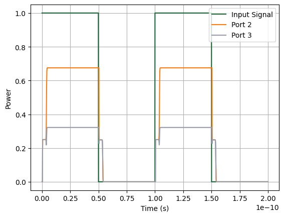
Interpreting the Time-Domain Output

At the very start, the outputs are almost identical, showing only a small shift due to the short delay through the straight arm.

This is why both outputs track each other right after the input changes.

Once the signal traveling through the spiral delay line arrives—after a larger delay—the two optical paths recombine with a relative phase difference.

This phase difference causes interference, leading to the characteristic constructive and destructive output pattern of an MZI.

Important: In this example the instantaneous phase difference \(\Delta\phi(t)\) is not exactly \(0\) or \(\pi\), so we do not observe full transmission or perfect extinction. Instead, the outputs settle at partial contrast: \(P_2 \propto 1 + \cos\Delta\phi,\quad P_3 \propto 1 - \cos\Delta\phi,\)

In summary:

1. Small initial delay → outputs look the same.

2. Larger spiral-induced delay → interference starts, splitting power between the two output ports, with partial (not complete) constructive/destructive interference.

Activating Tidy3D for High-Accuracy Simulation

We switch the directional coupler and spiral bends to use their Tidy3D full-wave models, enabling more accurate simulations that capture electromagnetic effects beyond analytical approximations.

# Use Tidy3D model for bends inside spiral
spiral.update(bend_kwargs={"active_model": "Tidy3D"})

# Use Tidy3D model for directional coupler
directional_coupler.activate_model("Tidy3D")

.venv/photonforge/lib/python3.13/site-packages/photonforge/parametric.py:1672: RuntimeWarning: Arguments 'active_model', 'tidy3d_model_kwargs', and 'waveguide_model_kwargs' are deprecated. Please use argument 'model' instead.
  bend0 = _bend(**bend_kwargs)
.venv/photonforge/lib/python3.13/site-packages/photonforge/parametric.py:1674: RuntimeWarning: Arguments 'active_model', 'tidy3d_model_kwargs', and 'waveguide_model_kwargs' are deprecated. Please use argument 'model' instead.
  bend1 = _bend(**bend_kwargs)

Tidy3DModel(run_time=None, medium=None, symmetry=(0, 0, 0), boundary_spec=None, monitors=(), structures=(), grid_spec=None, shutoff=None, subpixel=None, courant=None, port_symmetries=(), bounds=((None, None, None), (None, None, None)), source_gap=None, simulation_updates={}, verbose=True)

After activating the high-fidelity models, we re-initialize the MZI’s time-stepper for time-domain simulation. We also reduce rms_error_tolerance to suppress warnings that occur when the pole-residue fit error exceeds this value. While increasing the Tidy3D simulation accuracy would also prevent this warning, the current setting provides sufficient accuracy for the final results.

# Setting rms_error_tolerance for pole-residue fit
pf.config.default_time_steppers['*'] = pf.SMatrixTimeStepper(rms_error_tolerance=0.001)

# Set up time stepper
ts_td = mzi.setup_time_stepper(
    time_step=time_step,
    carrier_frequency=f_c,
    time_stepper_kwargs={
        "frequencies": np.linspace(f_c - 200 * f_m, f_c + 200 * f_m, 100),
    },
)

# Reset the time-stepper to ensure a clean simulation start
ts_td.reset()

# Run the simulation for the given input waveforms
outputs_td = ts_td.step(inputs)

Progress: 100%
Progress: 2000/2000

plt.plot(t, np.abs(A1_in) ** 2, label="Input Signal")
plt.plot(t, np.abs(outputs_td["P2@0"]) ** 2, label="Port 2")
plt.plot(t, np.abs(outputs_td["P3@0"]) ** 2, label="Port 3")

# Labels and legend
plt.xlabel("Time (s)")
plt.ylabel("Power")
plt.legend(loc="upper right")
plt.grid(True)
plt.show()

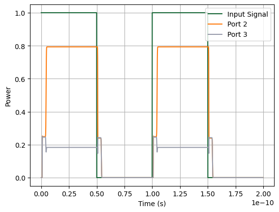
Why Do the Time-Domain Results Differ Between the Analytic and Tidy3D Models?

When using the Tidy3D model for bends, the full-wave solver captures subtle effects that are not included in the analytic bend model.

In particular, the effective index in the bend region differs slightly from that of a straight waveguide, which changes the optical phase accumulated along each arm of the MZI.

These phase changes lead to:

• A shift in the interference spectrum of the MZI.

• Corresponding changes in the S-matrix at a given frequency (both phase and amplitude can be affected).

• A different time-domain output waveform when driven with the same input.