Time-Domain Simulation of a Mach–Zehnder Modulator

Mach–Zehnder modulators (MZMs) are a core building block of high-speed optical transmitters. They modulate a continuous-wave (CW) optical carrier by splitting light into two arms, applying a voltage-controlled phase shift in one (or both) arms, and recombining the fields in an output coupler.

In this example, we build a compact, time-domain MZM testbench using PhotonForge:

• Couplers: DirectionalCouplerModel (frequency-domain S-parameters internally converted to time domain during simulation)

• Phase shifter: AnalyticWaveguideModel + PhaseModTimeStepper (length-aware phase modulation, optional voltage-dependent loss, optional RC bandwidth)

• Electrical drive: WaveformTimeStepper generating an NRZ PRBS waveform

• Optical excitation: CWLaserTimeStepper (no detuning; laser frequency equals the carrier)

import numpy as np
import photonforge as pf
from matplotlib import pyplot as plt
from photonforge.live_viewer import LiveViewer

viewer = LiveViewer()

LiveViewer started at http://localhost:34523

Configuration and parameters

PhotonForge can simulate circuits built from schematic components (no layout geometry) by wiring subcomponents through virtual ports.

• Optical virtual ports represent optical mode amplitudes.

• Electrical virtual ports represent electrical wave amplitudes.

These virtual ports let us assemble a circuit graph and run time-domain propagation without requiring physical port locations or routing.

# Set the default technology
pf.config.default_technology = pf.basic_technology()

# Virtual port specs (schematic wiring)
opt_vir = pf.virtual_port_spec(classification="optical")
elec_vir = pf.virtual_port_spec(classification="electrical")

Silicon PN-depletion MZM parameters

We choose a set of typical starting parameters for a lumped PN-depletion phase shifter in silicon.

Note (lumped vs. travelling-wave EO drive):

This tutorial uses PhaseModTimeStepper, which models a lumped electro-optic phase modulator: the electrical drive is applied uniformly along the device and the travelling RF wave / transmission-line effects are neglected (no distributed RF propagation, reflections, or velocity mismatch).

To include a travelling-wave electrode model with a terminated transmission line, use TerminatedModTimeStepper.

Phase modulation figure of merit

PhaseModTimeStepper uses the standard length-aware phase law:

\[\Delta\phi(t) = \frac{\pi\,V(t)\,\ell}{V_{\pi L}}\]

• \(\ell\): phase shifter length

• \(V_{\pi L}\): efficiency in units of V·length (here V·μm)

• The corresponding half-wave voltage is \(V_{\pi} = V_{\pi L}/\ell\)

For an MZM biased near quadrature (maximum slope), a common choice is:

\[V_{\mathrm{bias}} \approx \frac{V_{\pi}}{2}\]

Loss and bandwidth knobs

This example also includes:

• Propagation loss specified in dB/μm.

• Optional voltage-dependent loss (linear coefficient).

• A simple RC-limited electrical bandwidth model via a first-order low-pass filter with time constant \(\tau_{\mathrm{RC}} = 1/(2\pi f_{\mathrm{RC}})\).

# Optical carrier (1550 nm)
lambda0 = 1.55
f_c = pf.C_0 / lambda0

# NRZ bit-rate (Hz)
bit_rate = 25e9

# Electrical port impedance used by PhaseModTimeStepper to convert field -> volts
Z0 = 50.0  # ohm

# Phase shifter (silicon PN depletion) parameters
length_um = 500.0  # 0.5 mm
n_eff = 2.4
n_group = 4.0

# V_piL in V·um (high pergood depletion modulators ~ 1 V·cm => 10000 V·um)
v_piL = 10000.0  # 1 V·cm

# Loss (dB/um). Example: 15 dB/cm => 15 * 1e-4 dB/um
propagation_loss = 15.0e-4  # dB/um

# Voltage-dependent loss (small; dB/um/V)
dloss_dv = 0.5e-4  # 0.5 dB/cm/V

# RC-limited electrical bandwidth (Hz)
f_rc = 20e9
tau_rc = 1.0 / (2 * np.pi * f_rc + 1e-30)

Quadrature bias point

The MZM output depends on the differential phase between the two arms. For the arm that contains the phase shifter, the total optical phase at the carrier wavelength \(\lambda_0\) can be written as

\[\phi(V) = \underbrace{\frac{2\pi n_\mathrm{eff}\,\ell}{\lambda_0}}_{\phi_0\ \text{(static phase at }V=0\text{)}} \;+\; \underbrace{\frac{\pi V \ell}{V_{\pi L}}}_{\Delta\phi(V)\ \text{(EO phase shift)}}\]

Quadrature operation corresponds to a differential phase of

\[\phi(V_\mathrm{bias}) = \frac{\pi}{2} + m\pi,\qquad m\in\mathbb{Z}\]

where the integer \(m\) accounts for the fact that phase is defined modulo \(\pi\) for intensity transfer. Solving for \(V_\mathrm{bias}\) gives

\[V_\mathrm{bias} = \frac{V_{\pi L}}{\pi \ell}\left[\left(\frac{\pi}{2}+m\pi\right) - \phi_0\right]\]

In code, we pick \(m\) to shift the target phase \((\pi/2 + m\pi)\) close to \(\phi_0\) (so the resulting bias voltage is in a practical range):

# Bias / drive voltages (NRZ levels)
m = int(2 * n_eff * length_um / lambda0)
phi0 = 2 * np.pi * n_eff * length_um / lambda0
V_bias = (v_piL / (np.pi * length_um)) * ((np.pi / 2 + m * np.pi) - phi0)

V_pp = 2.0  # volts, peak-to-peak between NRZ levels
V_low = V_bias - V_pp / 2
V_high = V_bias + V_pp / 2

(V_bias, V_low, V_high)

(2.2580645161361805, 1.2580645161361805, 3.2580645161361805)

Directional couplers

We model the MZM input/output splitters using the built-in DirectionalCouplerModel. This is naturally a frequency-domain (S-matrix) component.

During a time-domain simulation, PhotonForge automatically converts frequency-domain components into an equivalent time-domain representation (internally using a poles-and-residues fit over the provided frequency grid). This lets us freely combine:

• compact time-domain models (the EO phase shifter), and

• frequency-domain S-matrix models (the couplers)

in a single circuit simulation.

directional_coupler = pf.DirectionalCouplerModel().black_box_component(opt_vir)
viewer(directional_coupler)

Electro-optic phase shifter

We now build the active device in the MZM arm: a two-port optical phase shifter with a single electrical drive port.

Why two objects?

We combine:

• AnalyticWaveguideModel: provides a compact waveguide model (effective index, group index, loss, etc.).

• PhaseModTimeStepper: provides the time-domain modulation law (voltage-to-phase, optional voltage-dependent loss, and optional RC filtering of the electrical input).

Phase and voltage conventions

The phase modulation law is:

\[\Delta\phi(t) = \frac{\pi\,V(t)\,\ell}{V_{\pi L}}\]

In the time-domain circuit, the electrical input is represented as a (generally complex) wave amplitude \(A(t)\). PhaseModTimeStepper converts this to a physical voltage using the port impedance:

\[V(t) = \Re\{A(t)\}\,\sqrt{\Re\{Z_0\}}\]

In this tutorial we explicitly set z0 = 50 Ω so the mapping from waveform amplitude to volts is unambiguous.

# Compact model wrapper (frequency-domain view / parameters container)
ps_model = pf.AnalyticWaveguideModel(
    n_eff=n_eff,
    length=length_um,
    n_group=n_group,
    reference_frequency=f_c,
    v_piL=v_piL,
    propagation_loss=propagation_loss,
    dloss_dv=dloss_dv,
)

# Time-domain stepper for the EO phase modulation
ps_model.time_stepper = pf.PhaseModTimeStepper(
    n_eff=n_eff,
    length=length_um,
    n_group=n_group,
    v_piL=v_piL,
    z0=Z0,
    propagation_loss=propagation_loss,
    dloss_dv=dloss_dv,
    tau_rc=tau_rc,
)

# Schematic (virtual-port) component
phase_shifter = ps_model.black_box_component(opt_vir, name="EO_PhaseShifter")

# Add a virtual electrical drive port
phase_shifter.add_port(pf.Port((0.5, 0.5), -90, spec=elec_vir))

viewer(phase_shifter)

NRZ PRBS electrical drive

To drive the PN-depletion phase shifter, we create an electrical source component using a TerminationModel whose time-stepper is WaveformTimeStepper.

NRZ PRBS waveform

We use:

• waveform="trapezoid" to approximate an NRZ waveform with finite rise/fall time.

• prbs=7 to generate a pseudorandom bit sequence.

For this waveform type, the generated values range from offset to offset + amplitude.

Mapping “desired volts” to WaveformTimeStepper amplitude

The PhaseModTimeStepper consumes an electrical wave amplitude \(A(t)\) and converts it to voltage via:

\[V(t) = \Re\{A(t)\}\,\sqrt{\Re\{Z_0\}}\]

So if we want NRZ levels \(V_{\mathrm{low}}\) and \(V_{\mathrm{high}}\), we choose:

\[\texttt{offset} = \frac{V_{\mathrm{low}}}{\sqrt{Z_0}},\qquad \texttt{amplitude} = \frac{V_{\mathrm{high}} - V_{\mathrm{low}}}{\sqrt{Z_0}}\]

This is exactly what the next cell implements (with \(Z_0 = 50\,\Omega\)).

src_model = pf.TerminationModel()
src_model.time_stepper = pf.WaveformTimeStepper(
    frequency=bit_rate,
    amplitude=(V_high - V_low) / (Z0**0.5),
    offset=V_low / (Z0**0.5),
    waveform="trapezoid",
    width=1,
    rise=0.1,
    fall=0.1,
    prbs=7,
    seed=123,
)

nrz_source = src_model.black_box_component(elec_vir, name="NRZ_Source")
viewer(nrz_source)

Optical excitation (CW laser)

The time-domain solver operates on complex envelopes referenced to a carrier frequency. We excite the modulator with an ideal CW laser implemented as a termination component using CWLaserTimeStepper.

• No detuning: The laser frequency is automatically set to the carrier f_c.

• (Optional) The second input of the first coupler is intentionally kept dark by connecting a 0 W CW termination, which provides a well-defined boundary condition without injecting light.

This mirrors typical transmitter operation where a single laser feeds one input of the MZM.

# CW laser source (no detuning: frequency = f_c)
laser_model = pf.TerminationModel()
laser_model.time_stepper = pf.CWLaserTimeStepper(power=1e-3)
laser = laser_model.black_box_component(opt_vir, name="Laser")

# Dark termination for the unused optical input
laser_dark_model = pf.TerminationModel()
laser_dark_model.time_stepper = pf.CWLaserTimeStepper(power=0.0)
laser_dark = laser_dark_model.black_box_component(opt_vir, name="Laser_Dark")

viewer(laser)

MZM-circuit assembly

To make the example easy to reproduce and publish, we assemble the full testbench using a single netlist dictionary and component_from_netlist.

What goes into the netlist

The netlist declares:

• instances: the building blocks (couplers, phase shifter, electrical driver, laser, dark termination)

• connections / virtual connections: how their ports are wired together

• ports: which ports are exposed as the top-level interface

• models: a CircuitModel that enables circuit-level simulation

External interface

Because both the lasers and the NRZ driver are included as internal sources, the top-level component exposes only the two optical output ports. This is convenient for time-domain simulation: we can run ts.step(...) without providing any explicit input TimeSeries.

# Assemble whole circuit via netlist
netlist = {
    "name": "MZM_PhaseModTimeStepper_Testbench",
    "instances": {
        "in_dc": {"component": directional_coupler, "origin": (0, 0)},
        "out_dc": {"component": directional_coupler, "origin": (11, 0)},
        "ps": {"component": phase_shifter, "origin": (9, 1)},
        "drv": {"component": nrz_source, "origin": (9, -1.2)},
        "laser": {"component": laser, "origin": (-2.5, 0.8)},
        "dark": {"component": laser_dark, "origin": (-2.5, -0.8)},
    },
    "connections": [
        # Optical inputs
        (("laser", "P0"), ("in_dc", "P1")),
        (("dark", "P0"), ("in_dc", "P0")),
        # MZM arms
        (("ps", "P0"), ("in_dc", "P3")),
        (("out_dc", "P1"), ("ps", "P1")),
        # Electrical drive
        (("drv", "E0"), ("ps", "E0")),
    ],
    "virtual connections": [
        (("in_dc", "P2"), ("out_dc", "P0")),
    ],
    # Expose only optical outputs for now
    "ports": [("out_dc", "P2"), ("out_dc", "P3")],
    "models": [(pf.CircuitModel(), "Circuit")],
}

mzm_tb = pf.component_from_netlist(netlist)
viewer(mzm_tb)

Time-domain simulation

With the full testbench assembled, we obtain a circuit time-stepper and run the simulation.

Time-step selection

For NRZ at bit rate \(R_b\), a practical choice is to use a fixed number of samples per unit interval (UI):

\[\Delta t = \frac{1}{R_b\,N_{\mathrm{samp/UI}}}\]

Frequency grid for time-domain conversion

Frequency-domain components (the couplers) must be converted to time domain. The frequencies grid provided in time_stepper_kwargs defines the band used by the internal fitting/conversion. A simple and robust choice is a symmetric span around the carrier that covers the modulation sidebands.

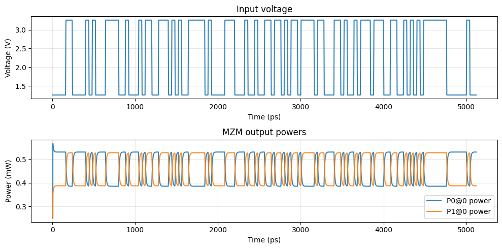
Outputs

The outputs are complex envelopes at the external optical ports. We plot output power as \(|A(t)|^2\) for both ports. We also add a monitor to the NRZ drive to extract input voltage and visualize it.

# Time grid: choose samples/bit and number of bits
samples_per_bit = 100
n_bits = 128

time_step = 1.0 / (bit_rate * samples_per_bit)
N_steps = int(n_bits * samples_per_bit)
t = time_step * np.arange(N_steps)

# Resolve subcomponent references for monitor placement
refs = mzm_tb.references
nrz_source_ref = refs[3]

# Build time-stepper (frequency grid used internally for fitting/conversion)
ts = mzm_tb.setup_time_stepper(
    time_step=time_step,
    carrier_frequency=f_c,
    time_stepper_kwargs={
        "frequencies": np.linspace(f_c - 200 * bit_rate, f_c + 200 * bit_rate, 100),
        "monitors": {"drive": nrz_source_ref["E0"]},
    },
)

# Run
ts.reset()
outputs = ts.step(steps=N_steps, time_step=time_step)

k0 = "P0@0"
k1 = "P1@0"
k2 = "drive@0+"

A0 = outputs[k0]
A1 = outputs[k1]
input_drive = outputs[k2]

P0 = np.abs(A0) ** 2
P1 = np.abs(A1) ** 2
v_in = np.real(input_drive) * np.sqrt(Z0)

Progress: 100%
Progress: 12800/12800

# Plot output powers
fig, ax = plt.subplots(2, 1, figsize=(10, 5))

ax[0].plot(t * 1e12, v_in, label="Input voltage", alpha=0.9)
ax[0].set_xlabel("Time (ps)")
ax[0].set_ylabel("Voltage (V)")
ax[0].set_title("Input voltage")
ax[0].grid(True, alpha=0.3)


ax[1].plot(t * 1e12, P0 * 1e3, label=f"{k0} power", alpha=0.9)
ax[1].plot(t * 1e12, P1 * 1e3, label=f"{k1} power", alpha=0.9)
ax[1].set_xlabel("Time (ps)")
ax[1].set_ylabel("Power (mW)")
ax[1].set_title("MZM output powers")
ax[1].grid(True, alpha=0.3)
ax[1].legend()

plt.tight_layout()
plt.show()