Optical Amplifier

Whenever a link runs out of power budget, an optical amplifier makes up the difference, and pays for it with amplified spontaneous emission (ASE). The OpticalAmplifierTimeStepper models a unidirectional amplifier with a constant power gain \(g\) (in dB) and ASE noise set by its noise figure through

\[S_\mathrm{ASE} = n_\mathrm{sp} \left( 10^{g/10} - 1 \right) h \nu \qquad n_\mathrm{sp} = \frac{10^{\mathrm{NF}/10}}{2}\]

where \(S_\mathrm{ASE}\) is the one-sided power spectral density of the noise added to the optical field. One interpretation detail matters when reading simulation results: the discrete-time simulation represents a spectral slice of width \(1 / \Delta t\) around the carrier, and the noise variance per sample is \(\sigma^2 = S_\mathrm{ASE} / \Delta t\), so the total ASE power in a simulation grows with its bandwidth. Optical signal-to-noise ratios extracted from a raw time series therefore refer to the simulation bandwidth; a receiver’s filters downstream select the noise that actually matters.

This guide verifies the gain and the ASE density, shows why amplifier placement in a lossy link matters, and closes with an amplified data signal.

Reference

1. Agrawal, G. P. Fiber-Optic Communication Systems. Wiley 2010.

Setup

import matplotlib.pyplot as plt
import numpy as np
import photonforge as pf
import photonforge.abstract as pfa

viewer = pf.live_viewer.LiveViewer()

LiveViewer started at http://localhost:51642

tech = pf.basic_technology()
pf.config.default_technology = tech

f0 = pf.C_0 / 1.55  # optical carrier at 1.55 um
h_planck = 6.62607015e-34  # Planck constant, used in the ASE formulas
time_step = 0.1e-12  # 0.1 ps step -> 10 THz simulation bandwidth

Gain and ASE Noise

The abstract optical_amplifier is a two-port device, amplifying from P0 to P1. With noise_figure=None (the default) it is a pure, noiseless gain block. Since most chains in this guide connect several two-port components in series, we use a small helper that strings components between a cw_laser and an exposed output port.

# 20 dB gain with a 5 dB noise figure; the seed makes the ASE reproducible
amplifier = pfa.optical_amplifier(gain=20, noise_figure=5, seed=0)
viewer(amplifier)

def run_chain(components, p_in, num_steps):
    # Connect the laser through each two-port component in order
    link = pf.Component("chain")
    laser_ref = link.add_reference(pfa.cw_laser(power=p_in))
    previous = laser_ref["P0"]
    for component in components:
        ref = link.add_reference(component)
        ref.connect("P0", previous)
        previous = ref["P1"]
    # Expose the end of the chain and run, returning the output field envelope
    link.add_port(previous, "out")
    link.add_model(pf.CircuitModel(), "Circuit")
    time_stepper = link.setup_time_stepper(
        time_step=time_step, carrier_frequency=f0, show_progress=False
    )
    return time_stepper.step(steps=num_steps, time_step=time_step, show_progress=False)["out@0"]

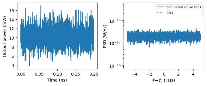
Amplifying a 0.1 mW carrier by 20 dB with a 5 dB noise figure shows both faces of the amplifier: the mean power comes out at exactly 10 mW, and the field now carries ASE fluctuations. Removing the mean field leaves the pure noise, whose spectral density is flat across the simulation bandwidth; the analytic \(S_\mathrm{ASE}\) from the formulas above is drawn for reference.

gain_db = 20
nf_db = 5
p_in = 1e-4  # 0.1 mW input carrier
num_steps = 2**16  # long record for a clean noise spectrum
t = np.arange(num_steps) * time_step

# Single amplifier fed by the CW laser
a = run_chain([pfa.optical_amplifier(gain=gain_db, noise_figure=nf_db, seed=0)], p_in, num_steps)

# Separate the amplified carrier from the ASE fluctuations
carrier = a.mean()
noise = a - carrier

# One-sided PSD of the complex noise field, averaged over segments
num_segments = 16
seg_len = num_steps // num_segments
psd = np.zeros(seg_len)
for k in range(num_segments):
    seg = noise[k * seg_len : (k + 1) * seg_len]
    psd += np.abs(np.fft.fftshift(np.fft.fft(seg))) ** 2 * time_step / seg_len
psd /= num_segments
freq = np.fft.fftshift(np.fft.fftfreq(seg_len, time_step))

# Analytic ASE spectral density: S_ASE = n_sp (G - 1) h f0, for reference
n_sp = 10 ** (nf_db / 10) / 2
s_ase = n_sp * (10 ** (gain_db / 10) - 1) * h_planck * f0

fig, (ax1, ax2) = plt.subplots(1, 2, figsize=(7, 3), tight_layout=True)
ax1.plot(t[:2000] * 1e9, np.abs(a[:2000]) ** 2 * 1e3)
ax1.set(xlabel="Time (ns)", ylabel="Output power (mW)")
ax2.semilogy(freq / 1e12, psd, label="Simulated noise PSD")
ax2.axhline(s_ase, color="k", linestyle=":", label="$S_{ASE}$")
ax2.set(xlabel="$f - f_0$ (THz)", ylabel="PSD (W/Hz)", ylim=(s_ase / 30, s_ase * 30))
ax2.legend(fontsize=8)

print(f"Mean output power: {np.abs(carrier)**2 * 1e3:.3f} mW "
      f"(input {p_in * 1e3:.1f} mW + {gain_db} dB)")
print(f"ASE power in the {1e-12 / time_step:.0f} THz simulation bandwidth: "
      f"{(np.abs(noise) ** 2).mean() * 1e3:.3f} mW")

Mean output power: 10.008 mW (input 0.1 mW + 20 dB)
ASE power in the 10 THz simulation bandwidth: 0.201 mW

Where to Amplify

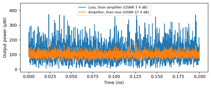
Because every amplifier adds the same ASE for a given gain and noise figure, its position in a lossy link decides how much that noise matters relative to the signal. The classic rule from cascade (Friis) analysis: amplify while the signal is still strong. We compare two chains with identical net gain, 10 dB of span loss followed by a 10 dB amplifier, and the same amplifier placed before the loss. A noiseless negative-gain amplifier serves as a convenient attenuator.

Both chains deliver the same mean power, but in the loss-first chain the full ASE lands on an attenuated signal, while in the amplify-first chain the loss attenuates the ASE together with the signal: the optical signal-to-noise ratio differs by exactly the span loss, 10 dB.

# A noiseless negative-gain amplifier is a clean 10 dB attenuator
attenuator = pfa.optical_amplifier(gain=-10, seed=1)
amplifier_10 = pfa.optical_amplifier(gain=10, noise_figure=5, seed=2)

# Same net gain (0 dB), different ordering of loss and amplification
chains = {
    "Loss, then amplifier": [attenuator, amplifier_10],
    "Amplifier, then loss": [amplifier_10, attenuator],
}

fig, ax = plt.subplots(figsize=(7, 3), tight_layout=True)
for label, chain in chains.items():
    a = run_chain(chain, p_in, num_steps)
    # Signal = mean field; ASE = mean power of the fluctuations around it
    signal_power = np.abs(a.mean()) ** 2
    ase_power = (np.abs(a - a.mean()) ** 2).mean()
    osnr_db = 10 * np.log10(signal_power / ase_power)
    ax.plot(t[:2000] * 1e9, np.abs(a[:2000]) ** 2 * 1e6, label=f"{label} (OSNR {osnr_db:.1f} dB)")
    print(f"{label}: signal {signal_power * 1e6:.1f} µW, "
          f"ASE {ase_power * 1e6:.2f} µW, OSNR {osnr_db:.1f} dB")

ax.set(xlabel="Time (ns)", ylabel="Output power (µW)")
_ = ax.legend(fontsize=8)

Loss, then amplifier: signal 99.9 µW, ASE 18.23 µW, OSNR 7.4 dB
Amplifier, then loss: signal 100.0 µW, ASE 1.82 µW, OSNR 17.4 dB

Amplified Data

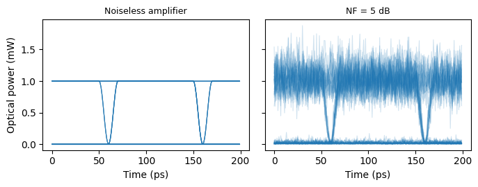
As a closing demonstration, an amplifier recovers a data signal at the end of a lossy link. A 10 Gb/s NRZ transmitter, built from a mach_zehnder_modulator biased at quadrature (phase_bias of 90°) and driven by a PRBS signal_source, launches 1 mW; the link attenuates it by 20 dB and a 20 dB preamplifier restores the level. Folding the received power into eye diagrams with the amplifier’s noise disabled and enabled shows the signal-ASE beat noise concentrating on the one level, the signature of optically preamplified receivers.

Here the simulation bandwidth point from the introduction becomes practical: with a 1 ps time step the simulated spectral slice is 1 THz wide, and all the ASE in it beats against the signal. A real receiver would follow the amplifier with an optical band-pass filter; in a simulation, either include such a filter explicitly or keep in mind that the time step sets the ASE bandwidth of the results.

bit_rate = 10e9
time_step_eye = 1e-12
unit_interval = int(round(1 / bit_rate / time_step_eye))  # samples per bit
num_bits = 128
t_eye = np.arange(2 * unit_interval) * time_step_eye  # eye spans two unit intervals
v_pi = 4.0
z0 = 50.0

# Same link twice: preamplifier without and with ASE noise
fig, axes = plt.subplots(1, 2, figsize=(7, 2.8), sharey=True, tight_layout=True)
for ax, noise_figure in zip(axes, [None, 5]):
    transmitter = pf.Component("amplified_link")
    laser_ref = transmitter.add_reference(pfa.cw_laser(power=1e-3))
    modulator_ref = transmitter.add_reference(
        pfa.mach_zehnder_modulator(v_pi=v_pi, phase_bias=90)
    )
    # NRZ drive swinging v_pi/2 around the quadrature point (amplitudes in V / sqrt(z0))
    source_ref = transmitter.add_reference(
        pfa.signal_source(
            frequency=bit_rate,
            amplitude=(v_pi / 2) / np.sqrt(z0),
            offset=(-v_pi / 4) / np.sqrt(z0),
            waveform="trapezoid",
            rise=0.1,
            fall=0.1,
            width=1.1,
            prbs=7,
            seed=0,
        )
    )
    # 20 dB span loss followed by a 20 dB preamplifier
    span_ref = transmitter.add_reference(pfa.optical_amplifier(gain=-20, seed=3))
    amplifier_ref = transmitter.add_reference(
        pfa.optical_amplifier(gain=20, noise_figure=noise_figure, seed=4)
    )
    # Chain in signal-flow order: laser -> MZM (driven by the source) -> span -> preamp
    modulator_ref.connect("P0", laser_ref["P0"])
    source_ref.connect("E0", modulator_ref["E0"])
    span_ref.connect("P0", modulator_ref["P1"])
    amplifier_ref.connect("P0", span_ref["P1"])
    transmitter.add_port(amplifier_ref["P1"], "out")
    transmitter.add_model(pf.CircuitModel(), "Circuit")

    num_steps = unit_interval * num_bits
    time_stepper = transmitter.setup_time_stepper(
        time_step=time_step_eye, carrier_frequency=f0, show_progress=False
    )
    output = time_stepper.step(steps=num_steps, time_step=time_step_eye, show_progress=False)
    power = np.abs(output["out@0"]) ** 2

    # Fold the received power into two-unit-interval segments to form the eye
    segments = power[unit_interval // 2 :]
    segments = segments[: len(segments) // (2 * unit_interval) * 2 * unit_interval]
    for segment in segments.reshape(-1, 2 * unit_interval):
        ax.plot(t_eye * 1e12, segment * 1e3, color="C0", alpha=0.2, linewidth=0.8)
    ax.set_title("Noiseless amplifier" if noise_figure is None else f"NF = {noise_figure} dB", fontsize=9)
    ax.set_xlabel("Time (ps)")
axes[0].set_ylabel("Optical power (mW)")
plt.show()

Summary

• pfa.optical_amplifier is a unidirectional two-port gain block: gain in dB, with ASE noise enabled by noise_figure (in dB) and disabled when it is None; seed makes noise realizations reproducible.

• The ASE spectral density follows \(S_\mathrm{ASE} = n_\mathrm{sp} (10^{g/10} - 1) h \nu\) with \(n_\mathrm{sp} = 10^{\mathrm{NF}/10} / 2\), and the per-sample noise variance is \(S_\mathrm{ASE} / \Delta t\): the simulation bandwidth \(1 / \Delta t\) acts as the ASE bandwidth, so noise powers read from raw time series scale with it.

• A negative gain with noise_figure=None makes a clean attenuator, handy for modeling span loss.

• Placement matters: amplifying before the loss preserves the optical signal-to-noise ratio, while amplifying after it costs exactly the span loss, the time-domain face of cascade noise analysis.

• On data signals, ASE appears as signal-spontaneous beat noise concentrated on the one level of the eye; the electrical counterpart of this block is the ElectricalAmplifierTimeStepper, and a pure optical noise source is available as the OpticalNoiseTimeStepper.