Semiconductor Optical Amplifier

A semiconductor optical amplifier (SOA) is a semiconductor waveguide whose core is an electrically pumped active region, typically InGaAsP quantum wells on InP. The injected carriers give the guide optical gain, and light is amplified in a single pass. SOAs are used as booster amplifiers after a transmitter, as preamplifiers before a receiver, and as gain sections in III-V and heterogeneously integrated photonic circuits.

The gain of an SOA depends on the optical power passing through it. Strong light consumes carriers faster than the pump current replaces them, so the gain falls: this is gain saturation. The carriers recover with the carrier lifetime \(\tau_c\), typically 100 ps to 500 ps, which is comparable to the bit period of a data signal. The gain at any instant therefore depends on the recent history of the signal. The carrier density also sets the refractive index, so every change of gain comes with a change of phase, which chirps the amplified light.

SemiconductorAmplifierTimeStepper models these effects together with amplified spontaneous emission (ASE), and semiconductor_amplifier wraps it in a two-port component that amplifies from P0 to P1. This guide shows how to use it for gain saturation under continuous-wave (CW) light, the amplification of short pulses, gain recovery, the pattern effect on non-return-to-zero (NRZ) data, and the chirp of amplified pulses. The constant-gain amplifier and the ASE noise model are covered in the Optical Amplifier guide.

What the time stepper computes

The model follows Agrawal and Olsson [1]. Let \(N\) be the carrier density in the active region, \(I\) the pump current, \(q\) the elementary charge and \(V\) the active volume. The carriers are supplied by the current, recombine with the lifetime \(\tau_c\) and are consumed by stimulated emission:

\[\frac{\partial N}{\partial t} = \frac{I}{qV} - \frac{N}{\tau_c} - \frac{g\,P}{h\nu\,\sigma},\]

where \(P\) is the optical power, \(h\nu\) the photon energy, \(\sigma\) the cross-section of the active region, and \(g\) the modal gain coefficient. Near transparency the gain is linear in the carrier density, \(g = \Gamma a\,(N - N_0)\), with \(\Gamma\) the confinement factor, \(a\) the differential gain and \(N_0\) the transparency density. Multiplying the rate equation by \(\Gamma a\) turns it into an equation for the gain itself:

\[\frac{\partial g}{\partial t} = \frac{g_0 - g}{\tau_c} - \frac{g\,P}{E_\mathrm{sat}}, \qquad E_\mathrm{sat} = \frac{h\nu\,\sigma}{a}.\]

Here \(g_0\) is the unsaturated gain set by the current and \(E_\mathrm{sat}\) is the saturation energy. The power grows along the device as \(\partial P/\partial z = g P\). Integrating the gain equation over the length \(L\) and writing \(h(t) = \int_0^L g\,\mathrm{d}z\) for the integrated gain, the term \(\int g P\,\mathrm{d}z\) becomes \(P_\mathrm{out} - P_\mathrm{in}\). With \(P_\mathrm{out} = e^h P_\mathrm{in}\) this gives a single ordinary differential equation, the one the time stepper integrates:

\[\frac{\mathrm{d}h}{\mathrm{d}t} = \frac{h_0 - h}{\tau_c} - \left(e^h - 1\right)\frac{P_\mathrm{in}(t)}{E_\mathrm{sat}}.\]

Time is measured in a frame that moves with the light, so the transit time through the device does not appear. The instantaneous power gain is \(G(t) = e^{h(t)}\).

The same carriers change the refractive index. The linewidth enhancement factor \(\alpha_H\), also called Henry’s factor, is the ratio of the index change to the gain change, and it makes the optical field acquire a phase \(-\alpha_H h/2\). The output field is

\[A_\mathrm{out}(t) = A_\mathrm{in}(t)\,\exp\!\left[\frac{h(t)}{2}\left(1 - j\alpha_H\right) \right],\]

with \(P = \lvert A \rvert^2\). ASE is added to the output with the one-sided spectral density \(S_\mathrm{ASE} = n_\mathrm{sp}\,(G - 1)\,h\nu\), as in the Optical Amplifier guide, but evaluated at the instantaneous gain \(G(t)\).

The component’s parameters map onto these quantities as follows:

• small_signal_gain is the unsaturated gain \(G_0 = e^{h_0}\), in dB.

• saturation_power is the internal saturation power \(P_\mathrm{sat} = E_\mathrm{sat}/\tau_c\), in W. Setting it to None disables saturation.

• carrier_lifetime is \(\tau_c\), in s.

• linewidth_enhancement_factor is \(\alpha_H\). A value of 0 disables the chirp.

• noise_figure is the noise figure NF in dB, which sets \(n_\mathrm{sp} = 10^{\mathrm{NF}/10}/2\). A value of None disables ASE.

The gain is spectrally flat around the carrier frequency, and effects faster than about a picosecond, such as carrier heating and spectral hole burning, are not included.

Reference

1. Agrawal, G. P., and Olsson, N. A. “Self-phase modulation and spectral broadening of optical pulses in semiconductor laser amplifiers.” IEEE Journal of Quantum Electronics 1989 25 (11), 2297-2306, doi: 10.1109/3.42059.

2. Connelly, M. J. Semiconductor Optical Amplifiers. Kluwer Academic Publishers 2002.

Setup

We use an InP SOA with 20 dB of small-signal gain, a 10 mW internal saturation power, a 200 ps carrier lifetime, \(\alpha_H = 5\) and a 7 dB noise figure. These are typical of a quantum-well SOA at 1550 nm. The saturation energy is then \(E_\mathrm{sat} = P_\mathrm{sat}\tau_c = 2\) pJ, which sets the scale for every pulse below.

import matplotlib.pyplot as plt
import numpy as np
import photonforge as pf
import photonforge.abstract as pfa

# Open the live viewer to display the amplifier component
viewer = pf.live_viewer.LiveViewer()

# Use the basic technology for the abstract components
pf.config.default_technology = pf.basic_technology()

# Set the optical carrier at 1550 nm (pf.C_0 is the speed of light in um/s)
f0 = pf.C_0 / 1.55

# Planck constant, used for the ASE photon energy
h_planck = 6.62607015e-34

# Set the amplifier parameters
g0_db = 20.0  # Small-signal gain (dB)
p_sat = 10e-3  # Internal saturation power (W)
tau_c = 200e-12  # Carrier lifetime (s)
alpha_h = 5.0  # Linewidth enhancement factor
nf_db = 7.0  # Noise figure (dB)

# Convert the small-signal gain to a linear power ratio
g0 = 10 ** (g0_db / 10)

# Compute the saturation energy E_sat = P_sat tau_c (J)
e_sat = p_sat * tau_c
print(f"Saturation energy: {e_sat * 1e12:.1f} pJ")

LiveViewer started at http://127.0.0.1:43807. Call its 'stop()' method to free the port.
Saturation energy: 2.0 pJ

Creating the amplifier

pfa.semiconductor_amplifier returns a two-port component that carries the time stepper. The component has no frequency-domain model, since a saturated gain depends on the signal and has no S matrix; it is used in time-domain simulations only.

# Create the SOA with gain saturation, chirp and ASE
soa = pfa.semiconductor_amplifier(
    small_signal_gain=g0_db,
    saturation_power=p_sat,
    carrier_lifetime=tau_c,
    linewidth_enhancement_factor=alpha_h,
    noise_figure=nf_db,
    seed=0,
)
viewer(soa)

A single component needs no surrounding circuit: setup_time_stepper returns its time stepper directly, and the input field is passed to step as a TimeSeries keyed by the input port, "P0@0". The output field is read from "P1@0". The field amplitudes are in \(\sqrt{\text{W}}\), so \(\lvert A \rvert^2\) is the power in watts.

With saturation and chirp disabled, the SOA reduces to the constant-gain optical_amplifier. The next cell drives both with the same weak CW input, 1 µW, and prints the output power and the ASE power per sample, which is \(S_\mathrm{ASE}/\Delta t\) for a time step \(\Delta t\).

time_step = 0.1e-12  # 0.1 ps step, a 10 THz simulation bandwidth
num_steps = 2**16  # Long record for a clean noise average
p_in = 1e-6  # CW input power: 1 uW

# Build the CW input field in sqrt(W)
a_in = np.full(num_steps, np.sqrt(p_in), dtype=complex)

# Create the two amplifiers with the same gain, noise figure and noise seed
amplifiers = {
    "optical_amplifier": pfa.optical_amplifier(gain=g0_db, noise_figure=nf_db, seed=0),
    "semiconductor_amplifier": pfa.semiconductor_amplifier(
        small_signal_gain=g0_db, noise_figure=nf_db, seed=0
    ),
}

for name, amplifier in amplifiers.items():
    # Run the amplifier's time stepper on the CW input
    time_stepper = amplifier.setup_time_stepper(
        time_step=time_step, carrier_frequency=f0, show_progress=False
    )
    a_out = time_stepper.step(
        inputs=pf.TimeSeries({"P0@0": a_in}, time_step), show_progress=False
    )["P1@0"]

    # Separate the amplified carrier from the ASE fluctuations
    carrier = a_out.mean()
    ase_power = np.mean(np.abs(a_out - carrier) ** 2)
    print(
        f"{name}: output power {np.abs(carrier) ** 2 * 1e6:.1f} uW, "
        f"ASE power {ase_power * 1e6:.1f} uW"
    )

# Compute the analytic ASE power per sample, S_ASE / time_step
n_sp = 10 ** (nf_db / 10) / 2
s_ase = n_sp * (g0 - 1) * h_planck * f0
print(f"S_ASE / time_step: {s_ase / time_step * 1e6:.1f} uW")

optical_amplifier: output power 101.7 uW, ASE power 317.6 uW
semiconductor_amplifier: output power 101.7 uW, ASE power 317.6 uW
S_ASE / time_step: 317.9 uW

Both components produce the same output, sample for sample: about 100 µW of amplified signal plus about 320 µW of ASE across the 10 THz simulation bandwidth. The rest of the guide turns on the effects that only the SOA has, and turns ASE off so that each effect can be seen on its own.

Gain saturation

Under constant input power the gain settles where \(\mathrm{d}h/\mathrm{d}t = 0\). With \(G = e^h\) the steady state is

\[G = G_0 \exp\!\left[-\frac{(G - 1)\,P_\mathrm{in}}{P_\mathrm{sat}}\right].\]

This is implicit in \(G\), but it can be solved for the input power instead, \(P_\mathrm{in} = P_\mathrm{sat}\ln(G_0/G)/(G - 1)\), which gives the analytic saturation curve directly: pick a gain, compute the input power, and multiply by the gain for the output power.

Datasheets quote the saturation output power \(P_\mathrm{out,3dB}\), the output power at which the gain has fallen 3 dB below \(G_0\). It is not the same quantity as the internal \(P_\mathrm{sat}\) of the model. Setting \(G = G_0/2\) in the steady state gives \(P_\mathrm{out,3dB} = \ln 2\;G_0/(G_0 - 2)\;P_\mathrm{sat}\), and the function saturation_output_power performs this conversion. To match a datasheet, adjust saturation_power until it returns the quoted value.

The next cell sweeps the CW input power from -40 dBm to +10 dBm. Each run lasts 2 ns, ten carrier lifetimes, so the gain has settled by the last sample.

time_step = 1e-12  # 1 ps step, small against the 200 ps carrier lifetime
num_steps = 2000  # 2 ns, ten carrier lifetimes

# Sweep the CW input power (dBm)
p_in_dbm = np.linspace(-40, 10, 26)
p_in = 1e-3 * 10 ** (p_in_dbm / 10)

# Create the SOA with gain saturation only
soa = pfa.semiconductor_amplifier(
    small_signal_gain=g0_db, saturation_power=p_sat, carrier_lifetime=tau_c
)

gain = []
for power in p_in:
    # Run each input power from the unsaturated state
    time_stepper = soa.setup_time_stepper(
        time_step=time_step, carrier_frequency=f0, show_progress=False
    )
    a_in = np.full(num_steps, np.sqrt(power), dtype=complex)
    a_out = time_stepper.step(
        inputs=pf.TimeSeries({"P0@0": a_in}, time_step), show_progress=False
    )["P1@0"]

    # Read the settled gain from the last sample
    gain.append(np.abs(a_out[-1]) ** 2 / power)
gain = np.array(gain)
p_out = gain * p_in

# Compute the analytic curve by choosing the gain and solving for the input power
g_analytic = np.linspace(g0 * 0.999, 2, 500)
p_in_analytic = p_sat * np.log(g0 / g_analytic) / (g_analytic - 1)
p_out_analytic = g_analytic * p_in_analytic

# Convert the internal saturation power to the 3 dB output saturation power
p_out_3db = pf.saturation_output_power(g0_db, p_sat)
print(f"3 dB output saturation power: {10 * np.log10(p_out_3db / 1e-3):.2f} dBm")

# Plot the simulated gain against output power, with the steady-state law
fig, ax = plt.subplots(figsize=(7, 3.2), tight_layout=True)
ax.plot(10 * np.log10(p_out / 1e-3), 10 * np.log10(gain), "o", label="Simulation")
ax.plot(
    10 * np.log10(p_out_analytic / 1e-3),
    10 * np.log10(g_analytic),
    "k:",
    label="Steady-state law",
)

# Mark the 3 dB gain compression point
ax.axhline(g0_db - 3, color="gray", lw=0.8)
ax.axvline(10 * np.log10(p_out_3db / 1e-3), color="gray", lw=0.8)
ax.set(xlabel="Output power (dBm)", ylabel="Gain (dB)", xlim=(-20, 14), ylim=(9, 21))
ax.legend()
plt.show()

3 dB output saturation power: 8.50 dBm

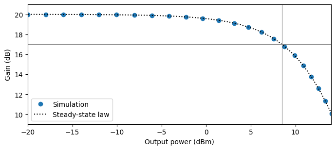
The gain stays at 20 dB while the output power is small against \(P_\mathrm{sat}\) and falls steeply once the output reaches a few milliwatts. The gray lines mark the 3 dB point: an internal saturation power of 10 mW (10 dBm) corresponds to a saturation output power of 8.5 dBm on a datasheet.

Amplifying short pulses

A pulse much shorter than \(\tau_c\) passes before the carriers can recover, so the relaxation term in the gain equation can be dropped during the pulse: \(\mathrm{d}h/\mathrm{d}t = -(e^h - 1)\,P_\mathrm{in}/E_\mathrm{sat}\). This equation integrates in closed form. With \(U(t) = \int_{-\infty}^t P_\mathrm{in}\,\mathrm{d}t'\) the input energy that has arrived by time \(t\),

\[1 - e^{-h(t)} = \left(1 - \frac{1}{G_0}\right) e^{-U(t)/E_\mathrm{sat}}.\]

The leading edge of the pulse sees the full gain \(G_0\), and every later part sees a gain already depleted by the energy ahead of it. Integrating \(e^h P_\mathrm{in}\) over the pulse gives the output energy for an input energy \(E_\mathrm{in}\) [1]:

\[E_\mathrm{out} = E_\mathrm{sat} \ln\!\left[1 + G_0\left(e^{E_\mathrm{in}/E_\mathrm{sat}} - 1\right)\right].\]

The energy gain \(E_\mathrm{out}/E_\mathrm{in}\) depends only on \(E_\mathrm{in}/E_\mathrm{sat}\) and not on the pulse shape. The next cell amplifies 10 ps Gaussian pulses with input energies from 0.001 \(E_\mathrm{sat}\) to 10 \(E_\mathrm{sat}\), and plots the energy gain with this law for reference.

time_step = 0.1e-12  # 0.1 ps step, 100 samples across the pulse
fwhm = 10e-12  # Pulse duration: full width at half maximum of the power (s)

# Set the time axis, with room after the pulse for the full output
t = np.arange(-100e-12, 400e-12, time_step)

# Build a Gaussian power shape that integrates to 1, so power = energy * shape
shape = np.exp(-4 * np.log(2) * (t / fwhm) ** 2)
shape /= shape.sum() * time_step

# Sweep the input pulse energy relative to the saturation energy
e_in = e_sat * np.logspace(-3, 1, 17)

# Pick three energies to plot the output pulse shape
shown = {1e-2: "C0", 1e-1: "C1", 1.0: "C2"}

fig, (ax1, ax2) = plt.subplots(1, 2, figsize=(7, 3), tight_layout=True)
e_out = []
for energy in e_in:
    # Run each pulse from the unsaturated state
    time_stepper = soa.setup_time_stepper(
        time_step=time_step, carrier_frequency=f0, show_progress=False
    )
    a_in = np.sqrt(energy * shape).astype(complex)
    a_out = time_stepper.step(
        inputs=pf.TimeSeries({"P0@0": a_in}, time_step), show_progress=False
    )["P1@0"]

    # Integrate the output power to get the output energy
    p_out = np.abs(a_out) ** 2
    e_out.append(p_out.sum() * time_step)

    # Plot the normalized output shape for the selected energies
    ratio = energy / e_sat
    for key, color in shown.items():
        if np.isclose(ratio, key):
            label = f"$E_{{in}}$ = {ratio:g} $E_{{sat}}$"
            ax1.plot(t * 1e12, p_out / p_out.max(), color=color, label=label)
e_out = np.array(e_out)

# Compute the closed-form energy gain for comparison
e_out_law = e_sat * np.log(1 + g0 * (np.exp(e_in / e_sat) - 1))

# Add the input pulse shape to the left panel
ax1.plot(t * 1e12, shape / shape.max(), "k:", label="Input")
ax1.set(xlabel="Time (ps)", ylabel="Normalized power", xlim=(-20, 20))
ax1.legend(fontsize=7)

# Plot the energy gain against the input energy in the right panel
ax2.semilogx(e_in / e_sat, 10 * np.log10(e_out / e_in), "o", label="Simulation")
ax2.semilogx(e_in / e_sat, 10 * np.log10(e_out_law / e_in), "k:", label="Closed form")
ax2.set(xlabel="$E_{in}$ / $E_{sat}$", ylabel="Energy gain (dB)")
ax2.legend(fontsize=7)
plt.show()

# Print the energy gain at the saturation energy
i_sat = np.argmin(np.abs(e_in - e_sat))
print(
    f"Energy gain at E_in = E_sat: {10 * np.log10(e_out[i_sat] / e_in[i_sat]):.2f} dB "
    f"(closed form {10 * np.log10(e_out_law[i_sat] / e_in[i_sat]):.2f} dB)"
)

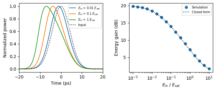
Energy gain at E_in = E_sat: 7.25 dB (closed form 7.12 dB)

The weakest pulses gain the full 20 dB, and the energy gain falls to 7.2 dB at \(E_\mathrm{in} = E_\mathrm{sat}\). The simulation sits about 0.1 dB above the closed form because a 10 ps pulse is 5% of the carrier lifetime, so the carriers recover slightly during the pulse, which the closed form neglects.

The left panel shows the cost in pulse shape. A strongly saturating pulse depletes the gain with its leading edge, so the trailing edge is amplified less: the output pulse is asymmetric and its peak moves earlier in time.

Gain recovery

After a pulse has passed, the gain returns to its unsaturated value. When the remaining input is weak, the extraction term is negligible and the gain equation reduces to \(\mathrm{d}h/\mathrm{d}t = (h_0 - h)/\tau_c\). The integrated gain, and so the gain in dB, recovers exponentially with the carrier lifetime.

A CW beam in the amplifier speeds this up. Linearizing the gain equation around a steady state with gain \(G\) under a CW power \(P_\mathrm{cw}\) gives an effective recovery time

\[\tau_\mathrm{eff} = \frac{\tau_c}{1 + G\,P_\mathrm{cw}/P_\mathrm{sat}},\]

because the extra stimulated emission pulls the carrier density back towards its steady state faster. Such a holding beam is a common way to make an SOA respond faster, at the cost of a lower steady-state gain.

The next cell sends a 2 pJ pulse, one saturation energy, through the SOA on top of a CW input of 1 µW and of 1 mW. The instantaneous gain is the ratio of output to input power. Each run starts 2 ns before the pulse so that the CW beam has settled the gain first.

time_step = 0.5e-12  # 0.5 ps step, 20 samples across the pulse

# Start 2 ns before the pulse so that the CW beam settles the gain
t = np.arange(-2000e-12, 1000e-12, time_step)

# Build the pump pulse: one saturation energy with a 10 ps duration
pulse = np.exp(-4 * np.log(2) * (t / fwhm) ** 2)
pulse *= e_sat / (pulse.sum() * time_step)

# Set the two CW powers with their plot labels
cw_powers = {1e-6: "CW power 1 µW", 1e-3: "CW power 1 mW"}

fig, ax = plt.subplots(figsize=(7, 3.2), tight_layout=True)
for p_cw, label in cw_powers.items():
    # Add the pulse on top of the CW beam
    a_in = np.sqrt(p_cw + pulse).astype(complex)

    # Run the SOA on the combined input
    time_stepper = soa.setup_time_stepper(
        time_step=time_step, carrier_frequency=f0, show_progress=False
    )
    a_out = time_stepper.step(
        inputs=pf.TimeSeries({"P0@0": a_in}, time_step), show_progress=False
    )["P1@0"]

    # Compute the instantaneous gain in dB
    gain_db = 10 * np.log10(np.abs(a_out) ** 2 / np.abs(a_in) ** 2)
    ax.plot(t * 1e12, gain_db, label=label)

    # Read the steady-state gain 100 ps before the pulse
    g_ss_db = gain_db[np.searchsorted(t, -100e-12)]

    # Compute the effective recovery time from the linearized gain equation
    tau_eff = tau_c / (1 + 10 ** (g_ss_db / 10) * p_cw / p_sat)

    # Find when the gain is back within 1 dB of its steady state
    i_min = np.argmin(gain_db)
    t_1db = t[i_min + np.argmax(gain_db[i_min:] > g_ss_db - 1)]
    print(
        f"{label}: steady-state gain {g_ss_db:.1f} dB, "
        f"tau_eff {tau_eff * 1e12:.0f} ps, within 1 dB after {t_1db * 1e12:.0f} ps"
    )

    # Draw the exponential recovery with tau_c after the pulse, for the weak CW input
    if p_cw == 1e-6:
        t_ref = t[t > 50e-12]
        g_start = gain_db[np.searchsorted(t, 50e-12)]
        decay = np.exp(-(t_ref - 50e-12) / tau_c)
        ax.plot(
            t_ref * 1e12, g0_db + (g_start - g0_db) * decay, "k:", label="$\\tau_c$ law"
        )

# Label the axes around the pulse and its recovery
ax.set(xlabel="Time (ps)", ylabel="Gain (dB)", xlim=(-100, 1000))
ax.legend()
plt.show()

CW power 1 µW: steady-state gain 20.0 dB, tau_eff 198 ps, within 1 dB after 577 ps
CW power 1 mW: steady-state gain 12.6 dB, tau_eff 71 ps, within 1 dB after 219 ps

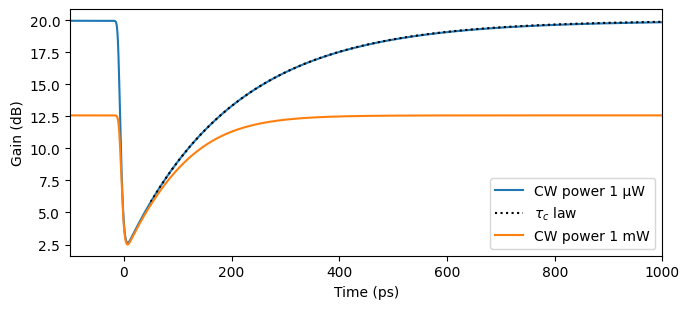
With the weak input the gain drops from 20 dB to 2.6 dB during the pulse and recovers along the exponential set by \(\tau_c\), taking about 580 ps to come back within 1 dB. The 1 mW holding beam lowers the steady-state gain to 12.6 dB and cuts the effective recovery time to 71 ps, so the gain is back within 1 dB after about 220 ps. Far from the steady state, just after the pulse, the recovery is slower than \(\tau_\mathrm{eff}\) predicts, because the linearization only holds close to the steady state.

Pattern effect on NRZ data

The gain responds to the signal with the time constant \(\tau_\mathrm{eff}\), so a data signal with a comparable bit period modulates the gain it passes through. A long run of zeros lets the gain recover, so the next one is amplified more; a long run of ones depletes the gain, so the last ones of the run are amplified less. This is the pattern effect, and it spreads the one level of the eye.

The next cell sends NRZ data with a 10 dB extinction ratio and a -10 dBm average input power, which drives the SOA 2.5 dB into compression, at 2.5 Gb/s and at 10 Gb/s. The bits are random, and the edges are smoothed with a Gaussian filter to give a realistic rise time. The output is normalized to its average power, so the two eyes can be compared directly.

time_step = 1e-12  # 1 ps step
num_bits = 512  # Number of random bits
num_skip = 16  # Bits discarded at the start while the gain settles
extinction_ratio_db = 10.0  # Ratio of the one to the zero power level (dB)
p_avg = 1e-4  # Average input power: -10 dBm
edge_fraction = 0.15  # Width of the edge-smoothing Gaussian, as a fraction of a bit

# Draw a reproducible random bit sequence
rng = np.random.default_rng(1)
bits = rng.integers(0, 2, num_bits)

# Map the bits to power levels with the chosen extinction ratio
levels = np.where(bits == 1, 1.0, 10 ** (-extinction_ratio_db / 10))

fig, axes = plt.subplots(1, 2, figsize=(7, 3), sharey=True, tight_layout=True)
for ax, bit_rate in zip(axes, [2.5e9, 10e9]):
    # Compute the number of samples per bit, the unit interval
    unit_interval = int(round(1 / bit_rate / time_step))

    # Hold each level for one bit, then smooth the edges with a Gaussian filter
    p_in = np.repeat(levels, unit_interval)
    width = edge_fraction * unit_interval
    k = np.arange(-4 * width, 4 * width + 1)
    kernel = np.exp(-0.5 * (k / width) ** 2)
    p_in = np.convolve(p_in, kernel / kernel.sum(), mode="same")

    # Scale the pattern to the chosen average power
    p_in *= p_avg / p_in.mean()

    # Run the SOA on the data signal
    time_stepper = soa.setup_time_stepper(
        time_step=time_step, carrier_frequency=f0, show_progress=False
    )
    a_out = time_stepper.step(
        inputs=pf.TimeSeries({"P0@0": np.sqrt(p_in).astype(complex)}, time_step),
        show_progress=False,
    )["P1@0"]

    # Normalize the output to its average power, skipping the settling bits
    p_out = np.abs(a_out[num_skip * unit_interval :]) ** 2
    p_out /= p_out.mean()

    # Fold the output into two-bit segments, centered on the bits, to form the eye
    segments = p_out[unit_interval // 2 :]
    segments = segments[: len(segments) // (2 * unit_interval) * 2 * unit_interval]
    t_eye = np.arange(2 * unit_interval) / unit_interval
    for segment in segments.reshape(-1, 2 * unit_interval):
        ax.plot(t_eye, segment, "C0", alpha=0.15, lw=0.8)
    ax.set(title=f"{bit_rate / 1e9:g} Gb/s", xlabel="Time (bits)")

    # Measure the spread of the one level at the bit centers
    centers = p_out[np.arange(num_bits - num_skip) * unit_interval + unit_interval // 2]
    ones = centers[bits[num_skip:] == 1]
    spread = 10 * np.log10(ones.max() / ones.min())
    print(f"{bit_rate / 1e9:g} Gb/s: one-level spread {spread:.2f} dB")

axes[0].set_ylabel("Normalized output power")
plt.show()

2.5 Gb/s: one-level spread 0.44 dB
10 Gb/s: one-level spread 1.65 dB

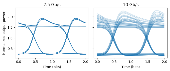
The two bit rates show the two faces of the pattern effect:

• At 2.5 Gb/s a bit lasts 400 ps, two carrier lifetimes. The gain recovers during each run of zeros and is depleted within the first part of each one, so every rising edge carries an overshoot, but the one level at the bit center is nearly the same for every bit.

• At 10 Gb/s a bit lasts 100 ps, shorter than \(\tau_\mathrm{eff}\). The gain carries the memory of several bits, so the one level depends on the preceding pattern and droops through each run of ones. The spread of the one level is about four times larger.

The pattern effect grows with compression. The next cell repeats the 10 Gb/s case over a range of average input powers and plots the spread of the one level against the average output power, with the 3 dB output saturation power marked. This is the curve that sets how hard an SOA booster can be driven for a given penalty.

bit_rate = 10e9
unit_interval = int(round(1 / bit_rate / time_step))

# Build the normalized 10 Gb/s pattern once, with smoothed edges
p_pattern = np.repeat(levels, unit_interval)
width = edge_fraction * unit_interval
k = np.arange(-4 * width, 4 * width + 1)
kernel = np.exp(-0.5 * (k / width) ** 2)
p_pattern = np.convolve(p_pattern, kernel / kernel.sum(), mode="same")
p_pattern /= p_pattern.mean()

# Sweep the average input power (dBm)
p_avg_dbm = np.arange(-30, 1, 2)
spread_db = []
p_out_avg = []
for power_dbm in p_avg_dbm:
    # Scale the pattern to this average power and run the SOA
    p_in = 1e-3 * 10 ** (power_dbm / 10) * p_pattern
    time_stepper = soa.setup_time_stepper(
        time_step=time_step, carrier_frequency=f0, show_progress=False
    )
    a_out = time_stepper.step(
        inputs=pf.TimeSeries({"P0@0": np.sqrt(p_in).astype(complex)}, time_step),
        show_progress=False,
    )["P1@0"]

    # Record the average output power and the spread of the one level
    p_out = np.abs(a_out[num_skip * unit_interval :]) ** 2
    p_out_avg.append(p_out.mean())
    centers = p_out[np.arange(num_bits - num_skip) * unit_interval + unit_interval // 2]
    ones = centers[bits[num_skip:] == 1]
    spread_db.append(10 * np.log10(ones.max() / ones.min()))

# Plot the one-level spread against the average output power
fig, ax = plt.subplots(figsize=(7, 3), tight_layout=True)
ax.plot(10 * np.log10(np.array(p_out_avg) / 1e-3), spread_db, "o-")

# Mark the 3 dB output saturation power
ax.axvline(10 * np.log10(p_out_3db / 1e-3), color="gray", lw=0.8)
ax.set(xlabel="Average output power (dBm)", ylabel="One-level spread (dB)")
plt.show()

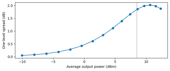
Below about -5 dBm of output power the one level spreads by less than 0.2 dB. The spread then grows quickly as the output approaches the saturation output power, marked in gray, where it reaches about 1.9 dB. Beyond that point it levels off near 2 dB and falls slightly: the deeper saturation shortens \(\tau_\mathrm{eff}\) below the 100 ps bit period, so the gain again settles within each bit, as it did at 2.5 Gb/s.

Chirp and spectral broadening

With \(\alpha_H \neq 0\) the output phase is \(\phi(t) = -\alpha_H h(t)/2\), so the phase follows the gain. The class uses the envelope convention in which a factor \(e^{-j 2\pi \Delta f\, t}\) in \(A(t)\) sits at the physical frequency \(f_0 + \Delta f\). The instantaneous frequency offset is therefore

\[\delta\nu(t) = -\frac{1}{2\pi}\frac{\mathrm{d}\phi}{\mathrm{d}t} = \frac{\alpha_H}{4\pi}\frac{\mathrm{d}h}{\mathrm{d}t},\]

and a spectrum computed with np.fft has to have its frequency axis reversed to read physical frequency. While a pulse depletes the gain, \(\mathrm{d}h/\mathrm{d}t < 0\) and the light shifts to lower frequencies, a red shift. Since the gain is depleted during the pulse and recovers only after it, the whole pulse is red-shifted, and the spectrum develops several peaks, the dominant one on the red side [1]. This is opposite to the blue-shifted trailing edge of Kerr self-phase modulation in a fiber.

The next cell amplifies 10 ps pulses of 0.1, 0.5 and 1 \(E_\mathrm{sat}\) with \(\alpha_H = 5\) and plots the instantaneous frequency across the pulse and the output spectra.

time_step = 0.1e-12  # 0.1 ps step, a 10 THz simulation bandwidth
t = np.arange(-200e-12, 600e-12, time_step)

# Build the Gaussian power shape, normalized to unit energy
shape = np.exp(-4 * np.log(2) * (t / fwhm) ** 2)
shape /= shape.sum() * time_step

# Create the SOA with gain saturation and chirp
soa_chirp = pfa.semiconductor_amplifier(
    small_signal_gain=g0_db,
    saturation_power=p_sat,
    carrier_lifetime=tau_c,
    linewidth_enhancement_factor=alpha_h,
)

# Reverse the FFT frequency axis to get the physical frequency offset (GHz)
freq = -np.fft.fftshift(np.fft.fftfreq(t.size, time_step)) / 1e9

fig, (ax1, ax2) = plt.subplots(1, 2, figsize=(7, 3), tight_layout=True)

# Plot the input spectrum for reference
spectrum_in = np.abs(np.fft.fftshift(np.fft.fft(np.sqrt(shape)))) ** 2
ax2.plot(freq, spectrum_in / spectrum_in.max(), "k:", label="Input")

for ratio in [0.1, 0.5, 1.0]:
    # Run the SOA on a pulse with this energy
    time_stepper = soa_chirp.setup_time_stepper(
        time_step=time_step, carrier_frequency=f0, show_progress=False
    )
    a_in = np.sqrt(ratio * e_sat * shape).astype(complex)
    a_out = time_stepper.step(
        inputs=pf.TimeSeries({"P0@0": a_in}, time_step), show_progress=False
    )["P1@0"]

    # Compute the instantaneous frequency offset from the output phase (GHz)
    phase = np.unwrap(np.angle(a_out))
    delta_nu = -np.gradient(phase, time_step) / (2 * np.pi) / 1e9
    label = f"{ratio:g} $E_{{sat}}$"
    within = np.abs(t) < 15e-12
    ax1.plot(t[within] * 1e12, delta_nu[within], label=label)

    # Compute the normalized output spectrum
    spectrum = np.abs(np.fft.fftshift(np.fft.fft(a_out))) ** 2
    ax2.plot(freq, spectrum / spectrum.max(), label=label)
    print(
        f"E_in = {ratio:g} E_sat: spectral peak at {freq[np.argmax(spectrum)]:.0f} GHz"
    )


# Label the frequency and spectrum panels
ax1.set(xlabel="Time (ps)", ylabel="Frequency offset (GHz)")
ax1.legend(fontsize=7)
ax2.set(xlabel="Frequency offset (GHz)", ylabel="Normalized spectrum", xlim=(-200, 100))
ax2.legend(fontsize=7)
plt.show()

E_in = 0.1 E_sat: spectral peak at -51 GHz
E_in = 0.5 E_sat: spectral peak at -90 GHz
E_in = 1 E_sat: spectral peak at -105 GHz

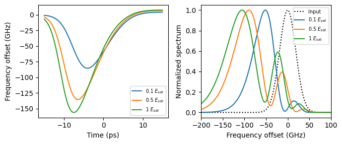
The instantaneous frequency falls across the leading half of the pulse, where the gain is being depleted fastest. It returns to zero on the trailing edge, where little gain is left to remove, and turns slightly positive after the pulse, where the gain starts to recover. The shift reaches more than 100 GHz for the stronger pulses. The spectra show the result: the main peak moves 50 GHz to 110 GHz to the red, and smaller peaks appear on its blue side. They arise because two instants within the pulse carry the same instantaneous frequency, and their contributions to the spectrum interfere.

This chirp matters whenever an SOA feeds a dispersive link or a narrow filter. A filter centered on the carrier frequency cuts the red-shifted light, and dispersion converts the chirp into pulse distortion.

Summary

• pfa.semiconductor_amplifier is a two-port SOA for time-domain simulations. Its gain follows the Agrawal and Olsson rate equation for the integrated gain \(h\), with the small-signal gain, the internal saturation power, the carrier lifetime, the linewidth enhancement factor and the noise figure as parameters.

• With saturation_power=None and linewidth_enhancement_factor=0 it is the constant-gain optical amplifier, including the same ASE noise.

• saturation_power is the internal saturation power of the model. Use pf.saturation_output_power to convert it to the 3 dB output saturation power quoted on datasheets.

• Pulses much shorter than the carrier lifetime are amplified according to their energy relative to \(E_\mathrm{sat} = P_\mathrm{sat}\tau_c\), and saturating pulses come out asymmetric.

• The gain recovers with the carrier lifetime, and faster with a CW holding beam, with the effective time \(\tau_c/(1 + G P_\mathrm{cw}/P_\mathrm{sat})\).

• On data, the finite recovery produces edge overshoot when the bit period is long against the recovery time and a pattern-dependent one level when it is short. The pattern effect grows steeply as the output approaches the saturation output power.

• A nonzero \(\alpha_H\) red-shifts saturating pulses and broadens their spectrum.