Custom Expressions

Not every electrical block in a circuit deserves a dedicated model: a mixer multiplies two drives, a driver amplifier saturates, a comparator snaps its input to logic levels. The ExpressionTimeStepper covers this long tail of custom signal processing: it is configured with one plain-text math expression per output port, and at every time step each output is the expression evaluated on the instantaneous inputs.

Several abstract components are ready-made instances of it:

Component	Ports	Operation
adder	E0, E1 → E2	\(s \, (w_0 E_0 + w_1 E_1)\)
multiplier	E0, E1 → E2	\(s \, E_0^{a} \, E_1^{b}\)
scaler	E0 → E1	\(s \, E_0\)
absolute	E0 → E1	\(s \, \vert E_0 \vert\)

The differentiator and integrator complete the electrical math family, but they are built on dedicated time steppers (DifferentialTimeStepper and IntegralTimeStepper) because they carry memory of past samples, which is precisely what an expression does not: the ExpressionTimeStepper is memoryless by construction.

This guide uses a ready-made block as an RF mixer and then builds two blocks from scratch: a saturating driver and a decision circuit.

The Expression Language

Expressions follow the syntax of the Expression class:

Constants	e, pi
Operators	+, -, *, /, %, ^ (exponent)
Math functions	abs, ceil, floor, exp, ln / log, log10, pow, sqrt
Trigonometric	sin, cos, tan, asin, acos, atan, atan2, sinh, cosh, tanh
Minimum/maximum	max, min (2 arguments each)
Conditionals	if(a, b, c), evaluating to b where a > 0 and c elsewhere; and(a, b); or(a, b)

A few rules govern how the expressions meet the component:

• The variables are the component’s electrical port names, written without the mode suffix (E0, not E0@0). Any electrical port without an expression outputs zero, and input ports can receive expressions too, which turns them into reflections: {"E0": "0.1 * E0"} gives port E0 a reflection coefficient of 0.1.

• Evaluation is instantaneous: each output sample is computed from the input samples of the same time step, with no internal state. Operations that require memory (delays, filtering, integration) are covered by DelayedTimeStepper, filter, and integrator.

• Like all electrical signals in the time-domain framework, the values are real wave amplitudes in \(\sqrt{\mathrm{W}}\), related to voltage by \(V = \Re \lbrace A \rbrace \sqrt{Z_0}\). Numeric constants inside an expression (thresholds, saturation levels) must be written in the same units; composing the strings with Python f-strings keeps that conversion explicit, as the examples below show.

Setup

import matplotlib.pyplot as plt
import numpy as np
import photonforge as pf
import photonforge.abstract as pfa

viewer = pf.live_viewer.LiveViewer()

LiveViewer started at http://localhost:53593

tech = pf.basic_technology()
pf.config.default_technology = tech

f0 = pf.C_0 / 1.55
time_step = 1e-12
z0 = 50.0  # impedance of the virtual electrical ports

A Ready-Made Block: Mixing Two Signals

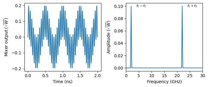
The multiplier computes the product of its two inputs, which is exactly what an ideal RF mixer does: for two sines at \(f_1\) and \(f_2\),

\[\sin(2 \pi f_1 t) \, \sin(2 \pi f_2 t) = \tfrac{1}{2} \cos \left( 2 \pi (f_1 - f_2) t \right) - \tfrac{1}{2} \cos \left( 2 \pi (f_1 + f_2) t \right),\]

the down- and up-converted products. Two signal_source components drive the multiplier: a 10 GHz local oscillator and a weaker 12 GHz tone standing in for a received signal. The output spectrum contains only the products at 2 GHz and 22 GHz, with nothing left at the original frequencies.

# Local oscillator and received tone (the seed only makes the components distinct)
lo_source = pfa.signal_source(waveform="sine", amplitude=1.0, frequency=10e9)
rf_source = pfa.signal_source(waveform="sine", amplitude=0.2, frequency=12e9, seed=1)

# Connect both sources to the multiplier inputs and expose its output
mixer = pf.Component("mixer")
lo_ref = mixer.add_reference(lo_source)
rf_ref = mixer.add_reference(rf_source)
multiplier_ref = mixer.add_reference(pfa.multiplier())
lo_ref.connect("E0", multiplier_ref["E0"])
rf_ref.connect("E0", multiplier_ref["E1"])
mixer.add_port(multiplier_ref["E2"], "out")
mixer.add_model(pf.CircuitModel(), "Circuit")

# 4 ns of simulation holds an integer number of cycles of every tone, for a clean spectrum
num_steps = 4000
t = np.arange(num_steps) * time_step

time_stepper = mixer.setup_time_stepper(
    time_step=time_step, carrier_frequency=f0, show_progress=False
)
# The circuit has no inputs: the zeros injected at the output port only set the duration
out = time_stepper.step(
    inputs=pf.TimeSeries({"out@0": np.zeros(num_steps)}, time_step), show_progress=False
)
mixed = np.real(out["out@0"])

# Single-sided amplitude spectrum
spectrum = np.abs(np.fft.rfft(mixed)) * 2 / num_steps
freq = np.fft.rfftfreq(num_steps, time_step)

fig, (ax1, ax2) = plt.subplots(1, 2, figsize=(7, 3), tight_layout=True)
ax1.plot(t[:2000] * 1e9, mixed[:2000])
ax1.set(xlabel="Time (ns)", ylabel=r"Mixer output ($\sqrt{W}$)")
ax2.plot(freq / 1e9, spectrum)
ax2.annotate("$f_1 - f_2$", (2, 0.1), xytext=(4, 0.1), fontsize=8, va="center")
ax2.annotate("$f_1 + f_2$", (22, 0.1), xytext=(24, 0.1), fontsize=8, va="center")
_ = ax2.set(xlabel="Frequency (GHz)", ylabel=r"Amplitude ($\sqrt{W}$)", xlim=(0, 30))

Building a Custom Block: a Saturating Driver

When none of the ready-made blocks fit, a custom one takes three steps:

1. create a Component and add electrical ports; virtual_port_spec provides port specifications that need no layout;

2. create a Model and store an ExpressionTimeStepper with the desired expressions in its time_stepper attribute; the base Model class serves as the carrier, since a nonlinear block has no S matrix to offer the frequency domain anyway;

3. add the model to the component.

The example is a driver amplifier that saturates, described by the standard soft-limiter model

\[V_\mathrm{out} = V_\mathrm{sat} \tanh \left( V_\mathrm{in} / V_\mathrm{sat} \right)\]

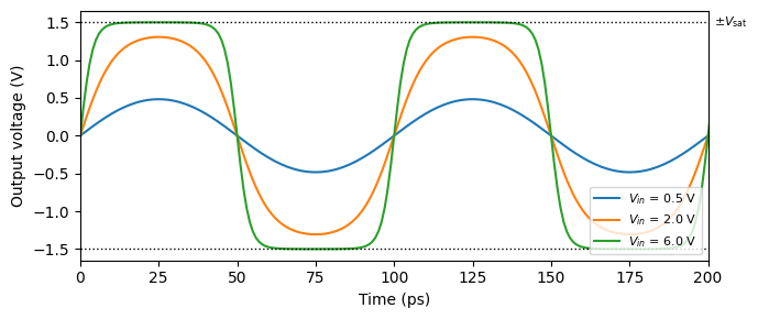
with \(V_\mathrm{sat} = 1.5\) V. The expression operates on wave amplitudes, so the saturation level is converted to \(a_\mathrm{sat} = V_\mathrm{sat} / \sqrt{Z_0}\) and embedded in the string with an f-string. Driving the block with 10 GHz sines of increasing amplitude shows the expected behavior: a small signal passes unchanged, while a large one flattens toward a square wave clipped at \(\pm V_\mathrm{sat}\).

v_sat = 1.5  # driver saturation voltage (V)
a_sat = v_sat / np.sqrt(z0)  # converted to a wave amplitude (√W)

# 1. Component with two virtual electrical ports (positions and angles are arbitrary)
port_spec = pf.virtual_port_spec(classification="electrical")
limiter = pf.Component("soft_limiter")
limiter.add_port(pf.Port((0, 0), 0, port_spec), "E0")
limiter.add_port(pf.Port((100, 0), 180, port_spec), "E1")

# 2. Base model carrying the expression stepper: E1 is the saturated copy of E0
model = pf.Model()
model.time_stepper = pf.ExpressionTimeStepper(
    expressions={"E1": f"{a_sat} * tanh(E0 / {a_sat})"}
)

# 3. Attach the model
limiter.add_model(model, "Limiter")

num_steps = 400
t = np.arange(num_steps) * time_step
time_stepper = limiter.setup_time_stepper(
    time_step=time_step, carrier_frequency=f0, show_progress=False
)

fig, ax = plt.subplots(figsize=(7, 3), tight_layout=True)
for v_in in [0.5, 2.0, 6.0]:
    # Drive amplitude converted from volts, injected directly at the input port
    drive = v_in / np.sqrt(z0) * np.sin(2 * np.pi * 10e9 * t)
    out = time_stepper.step(
        inputs=pf.TimeSeries({"E0@0": drive}, time_step), show_progress=False
    )
    # Output amplitude converted back to volts for plotting
    ax.plot(t * 1e12, np.real(out["E1@0"]) * np.sqrt(z0), label=f"$V_{{in}}$ = {v_in} V")
for level in (v_sat, -v_sat):
    ax.axhline(level, color="black", linestyle=":", linewidth=1)
ax.text(202, v_sat, r"$\pm V_\mathrm{sat}$", fontsize=8, va="center")
ax.set(xlabel="Time (ps)", ylabel="Output voltage (V)", xlim=(0, 200))
_ = ax.legend(fontsize=8, loc="lower right")

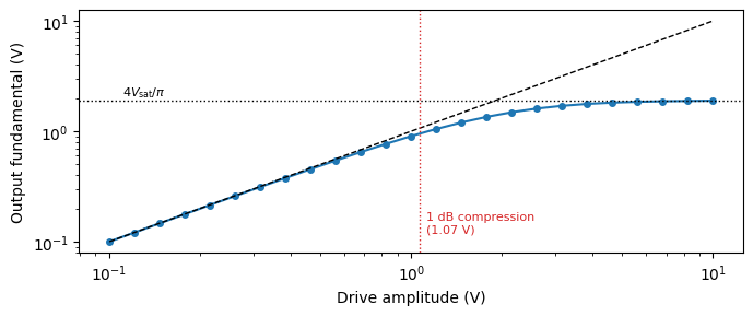
Sweeping the drive amplitude and extracting the fundamental at the output traces the gain compression curve, the standard characterization of a driver. At small drive the block is linear with unity gain; at large drive the output tends to a square wave of amplitude \(V_\mathrm{sat}\), whose fundamental \(4 V_\mathrm{sat} / \pi\) is the hard ceiling of the curve. The drive at which the output falls 1 dB below the linear extrapolation is the 1 dB compression point.

num_steps = 2000  # 20 cycles of the 10 GHz drive
t = np.arange(num_steps) * time_step
fundamental_bin = 20  # 10 GHz / (0.5 GHz frequency resolution)

v_in_sweep = np.logspace(-1, 1, 25)  # 0.1 V to 10 V
fundamental = []
for v_in in v_in_sweep:
    drive = v_in / np.sqrt(z0) * np.sin(2 * np.pi * 10e9 * t)
    out = time_stepper.step(
        inputs=pf.TimeSeries({"E0@0": drive}, time_step), show_progress=False
    )
    v_out = np.real(out["E1@0"]) * np.sqrt(z0)
    # Amplitude of the 10 GHz component of the output
    fundamental.append(np.abs(np.fft.rfft(v_out)[fundamental_bin]) * 2 / num_steps)
fundamental = np.array(fundamental)

# 1 dB compression: where the output drops to 10^(-1/20) of the linear extrapolation
gain = fundamental / v_in_sweep
v_1db = np.interp(-1.0, 20 * np.log10(gain[::-1]), v_in_sweep[::-1])

fig, ax = plt.subplots(figsize=(7, 3), tight_layout=True)
ax.loglog(v_in_sweep, fundamental, "o-", markersize=4, label="Output fundamental")
ax.loglog(v_in_sweep, v_in_sweep, "k--", linewidth=1, label="Linear (unity gain)")
ax.axhline(4 * v_sat / np.pi, color="black", linestyle=":", linewidth=1)
ax.text(0.11, 4 * v_sat / np.pi * 1.1, r"$4 V_\mathrm{sat} / \pi$", fontsize=8)
ax.axvline(v_1db, color="tab:red", linestyle=":", linewidth=1)
ax.text(v_1db * 1.05, 0.12, f"1 dB compression\n({v_1db:.2f} V)", fontsize=8, color="tab:red")
_ = ax.set(xlabel="Drive amplitude (V)", ylabel="Output fundamental (V)")

Conditional Logic: a Decision Circuit

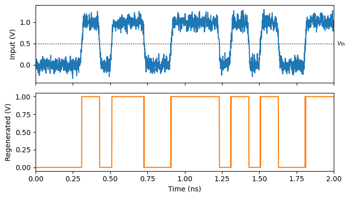
if(a, b, c) evaluates to b where a is positive and to c elsewhere, which is enough to build a comparator. The decision circuit at the end of a receiver chain snaps the degraded signal back to clean logic levels:

\[\begin{split}V_\mathrm{out} = \begin{cases} V_\mathrm{high} & V_\mathrm{in} > V_\mathrm{th} \\ 0 & \text{otherwise} \end{cases}\end{split}\]

Here a 10 Gb/s NRZ pattern with a 1 V swing and significant amplitude noise passes through a comparator with the threshold at mid-swing. The output is the regenerated pattern: clean levels, with the residual noise converted into edge timing errors where the noisy signal crosses the threshold.

v_high = 1.0  # logic-high output (V)
v_threshold = 0.5  # decision threshold (V)

# Comparator: same three-step recipe, with the conditional expression
comparator = pf.Component("decision_circuit")
comparator.add_port(pf.Port((0, 0), 0, port_spec), "E0")
comparator.add_port(pf.Port((100, 0), 180, port_spec), "E1")
model = pf.Model()
model.time_stepper = pf.ExpressionTimeStepper(
    expressions={
        "E1": f"if(E0 - {v_threshold / np.sqrt(z0)}, {v_high / np.sqrt(z0)}, 0)"
    }
)
comparator.add_model(model, "Comparator")

# Noisy 10 Gb/s NRZ pattern from the signal source
num_steps = 3200
t = np.arange(num_steps) * time_step
source = pfa.signal_source(
    waveform="trapezoid",
    amplitude=v_high / np.sqrt(z0),
    frequency=10e9,
    prbs=7,
    width=1.2,
    rise=0.2,
    fall=0.2,
    noise=2e-8,
    seed=7,
)
source_stepper = source.setup_time_stepper(
    time_step=time_step, carrier_frequency=f0, show_progress=False
)
noisy = np.real(
    source_stepper.step(
        inputs=pf.TimeSeries({"E0@0": np.zeros(num_steps)}, time_step), show_progress=False
    )["E0@0"]
)

# Regenerate the pattern through the comparator
time_stepper = comparator.setup_time_stepper(
    time_step=time_step, carrier_frequency=f0, show_progress=False
)
out = time_stepper.step(
    inputs=pf.TimeSeries({"E0@0": noisy}, time_step), show_progress=False
)
regenerated = np.real(out["E1@0"])

fig, (ax1, ax2) = plt.subplots(2, 1, figsize=(7, 4), sharex=True, tight_layout=True)
ax1.plot(t * 1e9, noisy * np.sqrt(z0))
ax1.axhline(v_threshold, color="black", linestyle=":", linewidth=1)
ax1.text(2.02, v_threshold, r"$V_\mathrm{th}$", fontsize=8, va="center")
ax1.set(ylabel="Input (V)")
ax2.plot(t * 1e9, regenerated * np.sqrt(z0), color="tab:orange")
_ = ax2.set(xlabel="Time (ns)", ylabel="Regenerated (V)", xlim=(0, 2))

Summary

• ExpressionTimeStepper turns plain-text math expressions into electrical signal-processing blocks: one expression per output port, evaluated sample by sample on the instantaneous inputs. Ports without an expression output zero, and expressions on input ports produce reflections.

• The abstract components adder, multiplier, scaler, and absolute are ready-made instances covering the common operations.

• A custom block takes three steps: a Component with virtual_port_spec electrical ports, a base Model whose time_stepper attribute holds the ExpressionTimeStepper, and add_model to attach it.

• Signals are wave amplitudes in \(\sqrt{\mathrm{W}}\) with \(V = \Re \lbrace A \rbrace \sqrt{Z_0}\); convert any constants in the expressions to the same units, most conveniently by composing the strings with f-strings.

• The stepper is memoryless by construction; combine it with DelayedTimeStepper, filter, differentiator, or integrator when the operation needs to remember past samples.