Photodiode

At the receiving end of every photonic link, a photodetector converts the optical signal back to the electrical domain. The PhotodiodeTimeStepper models a complete detection front-end for time-domain simulations: a photodiode followed by a transimpedance amplifier (TIA). The incident optical power \(P\) is converted to a photocurrent \(I = R P\) through the responsivity \(R\), then to the output voltage \(V = G R P\) through the TIA gain \(G\). At the electrical port, the voltage appears as the wave amplitude \(A = V / \sqrt{Z_0}\).

Beyond this ideal conversion, the model includes the main non-idealities of a real receiver: response bandwidth limits (first or second order), space-charge saturation in the photodiode, output saturation in the TIA, and shot, thermal, and pink noise.

This guide covers basic power detection, the square-law nature of the photodiode demonstrated with a heterodyne beat note, bandwidth limits, saturation, and detection noise.

Setup

import matplotlib.pyplot as plt
import numpy as np
import photonforge as pf
import photonforge.abstract as pfa

viewer = pf.live_viewer.LiveViewer()

LiveViewer started at http://localhost:51601

tech = pf.basic_technology()
pf.config.default_technology = tech

lda0 = 1.55
f0 = pf.C_0 / lda0
z0 = 50.0
q_e = 1.602176634e-19

Basic Detection

The easiest way to use the model is the photodiode component from the abstract library. It has one optical input P0 and one electrical output E0, and its time-domain behavior is the PhotodiodeTimeStepper. Here we set a responsivity of 0.8 A/W and keep the default TIA gain of 1 V/A.

responsivity = 0.8
photodiode = pfa.photodiode(responsivity=responsivity, seed=0)
viewer(photodiode)

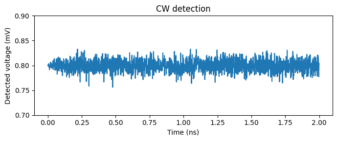
To detect something we need light: a 1 mW cw_laser is connected to the photodiode input, the electrical port is exposed, and a CircuitModel ties the circuit together for the time stepper. The detected voltage is recovered from the output wave amplitude as \(V = A \sqrt{Z_0}\).

The mean detected voltage matches \(V = G R P = 0.8\) mV, and the small ripple around it is the shot noise generated by the photodiode itself, to which we return in the last section.

laser = pfa.cw_laser(power=1e-3)

link = pf.Component("detection_link")
laser_ref = link.add_reference(laser)
photodiode_ref = link.add_reference(photodiode)
photodiode_ref.connect("P0", laser_ref["P0"])
link.add_port(photodiode_ref["E0"])
link.add_model(pf.CircuitModel(), "Circuit")

time_step = 1e-12
num_steps = 2000
t = np.arange(num_steps) * time_step

time_stepper = link.setup_time_stepper(time_step=time_step, carrier_frequency=f0)
output = time_stepper.step(steps=num_steps, time_step=time_step)
voltage = np.real(output["E0@0"]) * np.sqrt(z0)

fig, ax = plt.subplots(figsize=(7, 3), tight_layout=True)
ax.plot(t * 1e9, voltage * 1e3)
ax.set(xlabel="Time (ns)", ylabel="Detected voltage (mV)", ylim=(0.7, 0.9))
ax.set_title("CW detection")

print(f"Mean detected voltage: {voltage.mean() * 1e3:.3f} mV (expected {responsivity * 1e-3 * 1e3:.3f} mV)")

Mean detected voltage: 0.800 mV (expected 0.800 mV)

Square-Law Detection: Heterodyne Beat Note

The photodiode responds to optical power, not field amplitude. When two fields at different optical frequencies reach the detector, this square-law behavior mixes them: the detected power oscillates at the difference frequency. This is the basis of heterodyne detection and beat-note measurements.

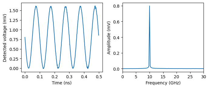
We combine two 1 mW lasers, one at the carrier frequency and one detuned by \(\Delta f = 10\) GHz, in a 3 dB directional_coupler. At one coupler output (the other is closed with an optical_termination), the detected power is

\[P(t) = \frac{P_1 + P_2}{2} + \sqrt{P_1 P_2} \cos(2 \pi \Delta f t + \varphi)\]

so the photocurrent should show a mean of \(R (P_1 + P_2)/2 = 0.8\) mA and a beat tone of amplitude \(R \sqrt{P_1 P_2} = 0.8\) mA at 10 GHz.

power_1 = power_2 = 1e-3
detuning = 10e9
laser_1 = pfa.cw_laser(power=power_1)
laser_2 = pfa.cw_laser(power=power_2, frequency=f0 + detuning)
photodiode = pfa.photodiode(responsivity=responsivity, seed=0)

heterodyne = pf.Component("heterodyne")
coupler_ref = heterodyne.add_reference(pfa.directional_coupler())
laser_1_ref = heterodyne.add_reference(laser_1)
laser_2_ref = heterodyne.add_reference(laser_2)
photodiode_ref = heterodyne.add_reference(photodiode)
termination_ref = heterodyne.add_reference(pfa.optical_termination())

laser_1_ref.connect("P0", coupler_ref["P0"])
laser_2_ref.connect("P0", coupler_ref["P1"])
photodiode_ref.connect("P0", coupler_ref["P2"])
termination_ref.connect("P0", coupler_ref["P3"])
heterodyne.add_port(photodiode_ref["E0"])
heterodyne.add_model(pf.CircuitModel(), "Circuit")

num_steps = 4096
t = np.arange(num_steps) * time_step

time_stepper = heterodyne.setup_time_stepper(time_step=time_step, carrier_frequency=f0)
voltage = np.real(time_stepper.step(steps=num_steps, time_step=time_step)["E0@0"]) * np.sqrt(z0)

spectrum = 2 * np.abs(np.fft.rfft(voltage - voltage.mean())) / num_steps
freq = np.fft.rfftfreq(num_steps, time_step)

fig, (ax1, ax2) = plt.subplots(1, 2, figsize=(7, 3), tight_layout=True)
ax1.plot(t[:500] * 1e9, voltage[:500] * 1e3)
ax1.set(xlabel="Time (ns)", ylabel="Detected voltage (mV)")
ax2.plot(freq / 1e9, spectrum * 1e3)
ax2.set(xlabel="Frequency (GHz)", ylabel="Amplitude (mV)", xlim=(0, 30))

peak = np.argmax(spectrum)
print(f"Beat tone at {freq[peak] / 1e9:.1f} GHz with amplitude {spectrum[peak] * 1e3:.3f} mV "
      f"(expected {responsivity * np.sqrt(power_1 * power_2) * 1e3:.3f} mV)")

Beat tone at 10.0 GHz with amplitude 0.798 mV (expected 0.800 mV)

Bandwidth

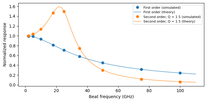
Real receivers do not respond instantly. The filter_frequency argument enables a first-order low-pass filter with the given 3 dB bandwidth. Setting filter_quality as well turns it into a second-order filter with natural frequency filter_frequency and the given quality factor, which produces gain peaking for \(Q > 1/\sqrt{2}\), a behavior typical of TIAs tuned for maximum flat bandwidth or intentional peaking.

The heterodyne setup gives us a direct way to trace the frequency response: sweeping the detuning of the second laser sweeps the beat frequency, and the detected tone amplitude at each point samples \(\lvert H(f) \rvert\). Since the components are parametric, we simply update the laser frequency in place and rerun the same circuit. The measured points follow the analytic first and second-order responses:

\[\lvert H_1(f) \rvert = \frac{1}{\sqrt{1 + (f / f_c)^2}} \qquad \lvert H_2(f) \rvert = \frac{1}{\sqrt{(1 - f^2 / f_c^2)^2 + f^2 / (Q f_c)^2}}\]

filter_frequency = 25e9
quality = 1.5
beat_freqs = np.array([2e9, 5e9, 10e9, 18e9, 25e9, 35e9, 50e9, 75e9, 100e9])
freq_fine = np.linspace(1e9, 110e9, 300)

theory = {
    "First order": (
        pfa.photodiode(responsivity=responsivity, filter_frequency=filter_frequency, seed=0),
        1 / np.sqrt(1 + (freq_fine / filter_frequency) ** 2),
    ),
    f"Second order, Q = {quality}": (
        pfa.photodiode(
            responsivity=responsivity,
            filter_frequency=filter_frequency,
            filter_quality=quality,
            seed=0,
        ),
        1 / np.sqrt(
            (1 - (freq_fine / filter_frequency) ** 2) ** 2
            + (freq_fine / (quality * filter_frequency)) ** 2
        ),
    ),
}

num_steps = 4096
t = np.arange(num_steps) * time_step
settled = slice(num_steps // 4, None)

fig, ax = plt.subplots(figsize=(7, 3.5), tight_layout=True)
for i, (label, (photodiode_bw, response_theory)) in enumerate(theory.items()):
    heterodyne_bw = pf.Component(f"heterodyne_bw_{i}")
    coupler_ref = heterodyne_bw.add_reference(pfa.directional_coupler())
    laser_1_ref = heterodyne_bw.add_reference(laser_1)
    laser_2_ref = heterodyne_bw.add_reference(laser_2)
    photodiode_ref = heterodyne_bw.add_reference(photodiode_bw)
    termination_ref = heterodyne_bw.add_reference(pfa.optical_termination())
    laser_1_ref.connect("P0", coupler_ref["P0"])
    laser_2_ref.connect("P0", coupler_ref["P1"])
    photodiode_ref.connect("P0", coupler_ref["P2"])
    termination_ref.connect("P0", coupler_ref["P3"])
    heterodyne_bw.add_port(photodiode_ref["E0"])
    heterodyne_bw.add_model(pf.CircuitModel(), "Circuit")

    measured = []
    for beat_freq in beat_freqs:
        laser_2.update(frequency=f0 + beat_freq)
        time_stepper = heterodyne_bw.setup_time_stepper(
            time_step=time_step, carrier_frequency=f0, show_progress=False
        )
        voltage = np.real(
            time_stepper.step(steps=num_steps, time_step=time_step, show_progress=False)["E0@0"]
        ) * np.sqrt(z0)
        tone = 2 * np.abs(
            np.mean(
                (voltage[settled] - voltage[settled].mean())
                * np.exp(-2j * np.pi * beat_freq * t[settled])
            )
        )
        measured.append(tone / (responsivity * np.sqrt(power_1 * power_2)))
    ax.plot(beat_freqs / 1e9, measured, "o", color=f"C{i}", label=f"{label} (simulated)")
    ax.plot(freq_fine / 1e9, response_theory, "-", color=f"C{i}", alpha=0.6, label=f"{label} (theory)")

ax.set(xlabel="Beat frequency (GHz)", ylabel="Normalized response")
_ = ax.legend(fontsize=8)

Saturation

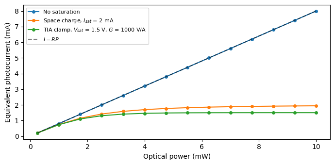
Two distinct mechanisms limit the output at high optical power. In the photodiode itself, space-charge screening compresses the photocurrent as it approaches saturation_current, with the sharpness of the transition set by roll_off. In the amplifier, the output voltage is clamped at saturation_voltage regardless of the input current.

We sweep the laser power through three receivers: an ideal one, one with a 2 mA space-charge saturation current, and one whose TIA clamps at 1.5 V (with a gain of 1000 V/A, corresponding to 1.5 mA of input current). Plotting the equivalent photocurrent \(V / G\) puts all three on the same axes.

receivers = {
    "No saturation": (pfa.photodiode(responsivity=responsivity, seed=0), 1.0),
    "Space charge, $I_{sat}$ = 2 mA": (
        pfa.photodiode(responsivity=responsivity, saturation_current=2e-3, seed=0),
        1.0,
    ),
    "TIA clamp, $V_{sat}$ = 1.5 V, $G$ = 1000 V/A": (
        pfa.photodiode(responsivity=responsivity, gain=1e3, saturation_voltage=1.5, seed=0),
        1e3,
    ),
}

powers = np.linspace(0.25e-3, 10e-3, 14)
num_steps = 2000

fig, ax = plt.subplots(figsize=(7, 3.5), tight_layout=True)
for label, (photodiode_sat, gain) in receivers.items():
    link_sat = pf.Component("link_" + label[:8])
    laser_ref = link_sat.add_reference(laser)
    photodiode_ref = link_sat.add_reference(photodiode_sat)
    photodiode_ref.connect("P0", laser_ref["P0"])
    link_sat.add_port(photodiode_ref["E0"])
    link_sat.add_model(pf.CircuitModel(), "Circuit")

    currents = []
    for power in powers:
        laser.update(power=power)
        time_stepper = link_sat.setup_time_stepper(
            time_step=time_step, carrier_frequency=f0, show_progress=False
        )
        voltage = np.real(
            time_stepper.step(steps=num_steps, time_step=time_step, show_progress=False)["E0@0"]
        ) * np.sqrt(z0)
        currents.append(voltage[num_steps // 4 :].mean() / gain)
    ax.plot(powers * 1e3, np.array(currents) * 1e3, "o-", markersize=4, label=label)

laser.update(power=1e-3)
ax.plot(powers * 1e3, responsivity * powers * 1e3, "k--", alpha=0.5, label="$I = R P$")
ax.set(xlabel="Optical power (mW)", ylabel="Equivalent photocurrent (mA)")
_ = ax.legend(fontsize=8)

Detection Noise

The model generates the fundamental noise sources of a receiver:

• Shot noise, with the one-sided current PSD \(S_I = 2 q I\), always present and growing with the detected current.

• Thermal noise of the TIA, set by thermal_noise as a one-sided input-referred current PSD in units of \(\mathrm{A^2 / Hz}\), independent of the optical power.

• Dark current (dark_current), which contributes its own shot noise even with no light.

• Pink noise, enabled by pink_noise_frequency, adding a \(1/f\) component below the given corner frequency.

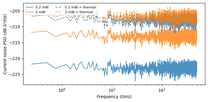
To see the first two, we measure the detected current noise PSD at two optical power levels, with and without a thermal noise of \((40\ \mathrm{pA}/\sqrt{\mathrm{Hz}})^2\). Shot noise moves up by 10 dB for a tenfold power increase, while the thermal floor does not: at 0.2 mW this receiver is thermally limited, and at 2 mW it approaches the shot-noise limit.

thermal_asd = 40e-12
cases = {
    "0.2 mW": (0.2e-3, 0.0),
    "2 mW": (2e-3, 0.0),
    "0.2 mW + thermal": (0.2e-3, thermal_asd**2),
    "2 mW + thermal": (2e-3, thermal_asd**2),
}

num_steps = 2**16
num_segments = 16
seg_len = num_steps // num_segments
freq = np.fft.rfftfreq(seg_len, time_step)

fig, ax = plt.subplots(figsize=(7, 3.5), tight_layout=True)
for i, (label, (power, thermal_noise)) in enumerate(cases.items()):
    photodiode_noise = pfa.photodiode(responsivity=responsivity, thermal_noise=thermal_noise, seed=0)
    link_noise = pf.Component(f"link_noise_{i}")
    laser_ref = link_noise.add_reference(laser)
    photodiode_ref = link_noise.add_reference(photodiode_noise)
    photodiode_ref.connect("P0", laser_ref["P0"])
    link_noise.add_port(photodiode_ref["E0"])
    link_noise.add_model(pf.CircuitModel(), "Circuit")

    laser.update(power=power)
    time_stepper = link_noise.setup_time_stepper(
        time_step=time_step, carrier_frequency=f0, show_progress=False
    )
    current = np.real(
        time_stepper.step(steps=num_steps, time_step=time_step, show_progress=False)["E0@0"]
    ) * np.sqrt(z0)

    psd = np.zeros(seg_len // 2 + 1)
    for k in range(num_segments):
        seg = current[k * seg_len : (k + 1) * seg_len]
        psd += 2 * np.abs(np.fft.rfft(seg - seg.mean())) ** 2 * time_step / seg_len
    psd /= num_segments

    style = "-" if thermal_noise == 0 else "--"
    color = f"C{i % 2}"
    ax.semilogx(freq[1:] / 1e9, 10 * np.log10(psd[1:]), style, color=color, alpha=0.8, label=label)
    theory = 2 * q_e * responsivity * power + thermal_noise
    print(f"{label}: measured {10 * np.log10(psd[1:].mean()):.1f} dB, "
          f"theory {10 * np.log10(theory):.1f} dB (A²/Hz)")

ax.set(xlabel="Frequency (GHz)", ylabel="Current noise PSD (dB A²/Hz)")
_ = ax.legend(fontsize=8, loc="upper left", ncols=2)

0.2 mW: measured -222.9 dB, theory -222.9 dB (A²/Hz)
2 mW: measured -212.9 dB, theory -212.9 dB (A²/Hz)
0.2 mW + thermal: measured -207.8 dB, theory -207.8 dB (A²/Hz)
2 mW + thermal: measured -206.8 dB, theory -206.8 dB (A²/Hz)

Summary

• pfa.photodiode models a photodiode plus TIA front-end: \(V = G R P\), exposed at the electrical port as the wave amplitude \(V / \sqrt{Z_0}\).

• Detection is square-law: fields at different optical frequencies mix into beat notes at their difference frequencies, which makes a two-laser heterodyne a convenient probe of the receiver.

• filter_frequency sets a first-order 3 dB bandwidth; adding filter_quality selects a second-order response with peaking for \(Q > 1/\sqrt{2}\).

• saturation_current and roll_off model space-charge compression of the photocurrent; saturation_voltage clamps the TIA output.

• Shot noise is always generated; thermal_noise (one-sided input-referred current PSD), dark_current, and pink_noise_frequency add the remaining receiver noise sources, and seed makes realizations reproducible.

• The optical sources used here are covered by the CWLaserTimeStepper; other abstract components, such as modulators and amplifiers, combine with the photodiode in the same way for full link simulations.