Ring Resonator

Micro-ring resonators pack narrow-band filtering, wavelength selectivity, and efficient modulation into tens of micrometers, which makes them ubiquitous in dense photonic circuits. They are also the components where time-domain simulation earns its keep: a high-Q cavity stores light for thousands of round trips, so its response to a modulated drive is dynamic, limited by the photon lifetime rather than by the electrical drive alone.

The RingTimeStepper simulates a single or double-bus ring as one bus coupler per waveguide plus a delay line for the round-trip propagation. Each coupler is the symmetric, lossless matrix with cross-coupling \(\kappa\) and through coefficient

\[\tau = -i e^{i \arg \kappa} \sqrt{1 - \lvert \kappa \rvert^2}\]

the same convention as the frequency-domain RingModel, covered in the Analytic Ring Model guide, so both models share resonance positions and line shapes. The model includes electro-optic and thermo-optic tuning of the ring index and loss, and an optional first-order low-pass filter on the electrical input.

This guide characterizes the ring spectrum from time-domain simulations, shows the cavity charging dynamics and their relation to the linewidth, and tunes the resonance thermally and electro-optically.

Setup

import matplotlib.pyplot as plt
import numpy as np
import photonforge as pf
import photonforge.abstract as pfa

viewer = pf.live_viewer.LiveViewer()

LiveViewer started at http://localhost:56397

tech = pf.basic_technology()
pf.config.default_technology = tech

z0 = 50.0

# Ring parameters: 60 µm round trip, silicon-like indices, 10 dB/cm loss
kappa = 0.117
length = 60.0
n_eff = 2.4
n_group = 4.2
loss = 1e-3

# Frequency at which n_eff is specified (1.55 µm)
f_ref = pf.C_0 / 1.55

The Ring Component

The abstract ring_resonator is a single-bus (all-pass) ring when only kappa1 is given, with ports P0 (input), P1 (through), and the electrical tuning port E0. We use a 60 µm round trip with \(n_g = 4.2\), giving a free spectral range \(\mathrm{FSR} = c_0 / (n_g \ell) \approx 1.19\) THz, and 10 dB/cm of propagation loss. The coupling \(\kappa = 0.117\) is chosen so that \(\lvert \tau \rvert\) equals the round-trip amplitude, the critical coupling condition where the transmission at resonance drops to zero.

ring = pfa.ring_resonator(
    kappa1=kappa, length=length, n_eff=n_eff, n_group=n_group, propagation_loss=loss
)
viewer(ring)

Spectral Response in the Time Domain

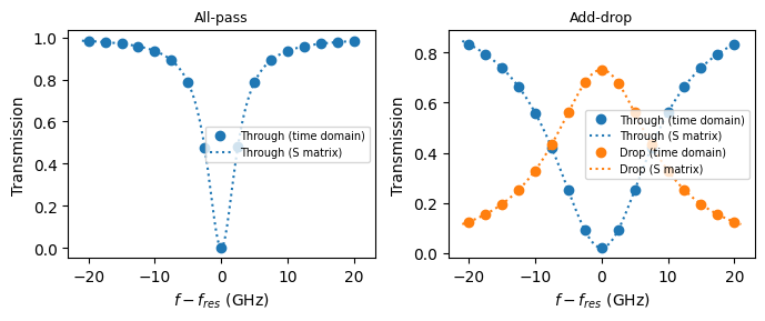
To trace the ring spectrum with the time stepper we sweep the laser frequency and record the steady-state transmission at each point. One detail deserves attention: the time stepper describes the ring at the simulation carrier frequency, and the resonance position of a ring with a mode number of a few hundred is extremely sensitive to the effective index. When the carrier moves, n_eff must move with it, consistently with the group index. For a constant \(n_g\), the effective index at frequency \(f\) is

\[n_\mathrm{eff}(f) = n_g + \left( n_\mathrm{eff}(f_\mathrm{ref}) - n_g \right) \frac{f_\mathrm{ref}}{f}\]

Since the component is parametric, each sweep point simply updates n_eff and reference_frequency together and reruns the same circuit. We also pick the time step as an integer fraction of the round-trip time, since the ring delay is implemented as a whole number of time steps.

The sweep is repeated for a double-bus (add-drop) ring, created by setting kappa2, which adds the P2 (drop) and P3 (add) ports. The component’s frequency-domain S matrix is used only to center each sweep on a resonance and to overlay the expected line shapes as dotted references.

def n_eff_at(f):
    # Effective index at frequency f, consistent with a constant group index
    return n_group + (n_eff - n_group) * f_ref / f

# The ring delay runs on whole time steps: make the round trip an exact multiple
round_trip = n_group * length / pf.C_0
time_step = round_trip / 42

# Settling time per sweep point (about 10 cavity lifetimes for this Q)
num_settle = 30000

# Double-bus version of the same ring for the drop-port response
ring_ad = pfa.ring_resonator(
    kappa1=0.2, kappa2=0.2, length=length, n_eff=n_eff, n_group=n_group, propagation_loss=loss
)

fsr = pf.C_0 / (n_group * length)
detunings = np.linspace(-20e9, 20e9, 17)
fig, (ax1, ax2) = plt.subplots(1, 2, figsize=(7, 3), tight_layout=True)

for ax, ring_dut, outputs in [
    (ax1, ring, {"P1": "Through"}),
    (ax2, ring_ad, {"P1": "Through", "P2": "Drop"}),
]:
    # Locate a resonance of this ring with the S matrix (coarse, then fine)
    ring_dut.update(n_eff=n_eff, reference_frequency=f_ref)
    freqs_c = np.linspace(f_ref - 0.6 * fsr, f_ref + 0.6 * fsr, 2001)
    t_c = np.abs(ring_dut.s_matrix(freqs_c, show_progress=False)[("P0@0", "P1@0")]) ** 2
    f_0 = freqs_c[np.argmin(t_c)]
    freqs_f = np.linspace(f_0 - 21e9, f_0 + 21e9, 1601)
    s_f = ring_dut.s_matrix(freqs_f, show_progress=False)
    t_f = np.abs(s_f[("P0@0", "P1@0")]) ** 2
    f_0 = freqs_f[np.argmin(t_f)]

    if ring_dut is ring:
        # Keep the all-pass resonance and linewidth for the following sections
        f_res = f_0
        half = (t_f.min() + 1) / 2
        in_band = freqs_f[t_f < half]
        fwhm = in_band.max() - in_band.min()

    measured = {port: [] for port in outputs}
    for detuning in detunings:
        # Re-reference the ring index to the new carrier before each run
        f_laser = f_0 + detuning
        ring_dut.update(n_eff=n_eff_at(f_laser), reference_frequency=f_laser)

        # Laser -> ring, with the unused electrical and add ports terminated
        link = pf.Component("sweep_link")
        laser_ref = link.add_reference(pfa.cw_laser(power=1e-3))
        ring_ref = link.add_reference(ring_dut)
        termination_ref = link.add_reference(pfa.electrical_termination())
        ring_ref.connect("P0", laser_ref["P0"])
        termination_ref.connect("E0", ring_ref["E0"])
        if "P3" in ring_dut.ports:
            add_termination_ref = link.add_reference(pfa.optical_termination())
            add_termination_ref.connect("P0", ring_ref["P3"])
        for port in outputs:
            link.add_port(ring_ref[port], "out_" + port)
        link.add_model(pf.CircuitModel(), "Circuit")

        # Let the cavity settle and read the steady-state output power
        time_stepper = link.setup_time_stepper(
            time_step=time_step, carrier_frequency=f_laser, show_progress=False
        )
        result = time_stepper.step(steps=num_settle, time_step=time_step, show_progress=False)
        for port in outputs:
            measured[port].append(np.abs(result[f"out_{port}@0"][-1]) ** 2 / 1e-3)

    for i, (port, label) in enumerate(outputs.items()):
        ax.plot(detunings / 1e9, measured[port], "o", color=f"C{i}", label=f"{label} (time domain)")
        ax.plot(
            (freqs_f - f_0) / 1e9,
            np.abs(s_f[("P0@0", f"{port}@0")]) ** 2,
            ":",
            color=f"C{i}",
            label=f"{label} (S matrix)",
        )
    ax.set(xlabel="$f - f_{res}$ (GHz)", ylabel="Transmission")
    ax.legend(fontsize=7)
ax1.set_title("All-pass", fontsize=9)
ax2.set_title("Add-drop", fontsize=9)

print(f"All-pass linewidth (S-matrix reference): {fwhm / 1e9:.2f} GHz, Q = {f_res / fwhm:,.0f}")

All-pass linewidth (S-matrix reference): 5.20 GHz, Q = 37,292

Cavity Charging and Ring-Down

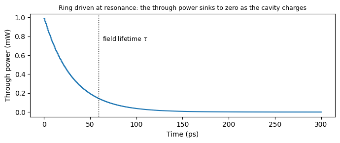
A resonator does not respond instantly. Starting the simulation with the cavity empty and the laser on resonance, the through-port power begins at the bare bus transmission and sinks toward the critically-coupled zero as the ring charges over many round trips. The transient decays with the cavity field lifetime \(\tau\), which is tied to the linewidth by \(\mathrm{FWHM} = 1 / (\pi \tau)\), so the same physics can be read in either domain.

# Drive the ring exactly on resonance, starting from an empty cavity
ring.update(n_eff=n_eff_at(f_res), reference_frequency=f_res)
link = pf.Component("ringdown_link")
laser_ref = link.add_reference(pfa.cw_laser(power=1e-3))
ring_ref = link.add_reference(ring)
termination_ref = link.add_reference(pfa.electrical_termination())
ring_ref.connect("P0", laser_ref["P0"])
termination_ref.connect("E0", ring_ref["E0"])
link.add_port(ring_ref["P1"], "out")
link.add_model(pf.CircuitModel(), "Circuit")

num_steps = 15000
t = np.arange(num_steps) * time_step
time_stepper = link.setup_time_stepper(
    time_step=time_step, carrier_frequency=f_res, show_progress=False
)
a = time_stepper.step(steps=num_steps, time_step=time_step)["out@0"]

# Fit the exponential decay of the field toward its steady state
residual = np.abs(a - a[-1]) / np.sqrt(1e-3)
window = (t > 10e-12) & (t < 150e-12)
slope = np.polyfit(t[window], np.log(residual[window]), 1)[0]
tau = -1 / slope

fig, ax = plt.subplots(figsize=(7, 3), tight_layout=True)
ax.plot(t * 1e12, np.abs(a) ** 2 * 1e3)
ax.axvline(tau * 1e12, color="k", linestyle=":", linewidth=1)
ax.text(tau * 1e12 + 4, 0.75, "field lifetime $\\tau$", fontsize=9)
ax.set(xlabel="Time (ps)", ylabel="Through power (mW)")
ax.set_title(
    "Ring driven at resonance: the through power sinks to zero as the cavity charges",
    fontsize=9,
)

print(f"Fitted field lifetime: {tau * 1e12:.1f} ps")
print(f"1 / (pi FWHM) from the reference spectrum: {1 / (np.pi * fwhm) * 1e12:.1f} ps")

Fitted field lifetime: 59.0 ps
1 / (pi FWHM) from the reference spectrum: 61.2 ps

Thermal Tuning

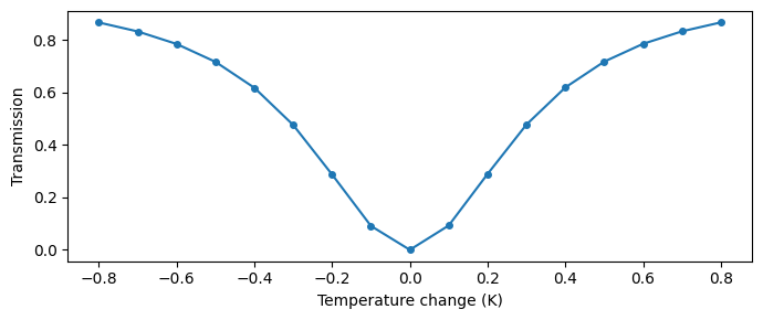
Rings are usually stabilized and tuned with integrated heaters. The dn_dT coefficient (with temperature and reference_temperature) shifts the ring index thermally; for silicon, \(\mathrm{d}n / \mathrm{d}T \approx 1.8 \times 10^{-4}\) /K moves the resonance by \(f \, (\mathrm{d}n / \mathrm{d}T) / n_g \approx 8\) GHz/K. Sweeping the temperature with the laser fixed on the cold resonance walks the resonance through the laser, tracing the (mirrored) line shape in temperature.

dn_dt = 1.8e-4

# Same ring, but with a thermo-optic coefficient and referenced at the laser
ring_thermal = pfa.ring_resonator(
    kappa1=kappa,
    length=length,
    n_eff=n_eff_at(f_res),
    reference_frequency=f_res,
    n_group=n_group,
    propagation_loss=loss,
    dn_dT=dn_dt,
)

temperatures = 293 + np.linspace(-0.8, 0.8, 17)
transmission = []
for temperature in temperatures:
    # Update the operating temperature and rerun the same circuit
    ring_thermal.update(temperature=temperature)
    link = pf.Component("thermal_link")
    laser_ref = link.add_reference(pfa.cw_laser(power=1e-3))
    ring_ref = link.add_reference(ring_thermal)
    termination_ref = link.add_reference(pfa.electrical_termination())
    ring_ref.connect("P0", laser_ref["P0"])
    termination_ref.connect("E0", ring_ref["E0"])
    link.add_port(ring_ref["P1"], "out")
    link.add_model(pf.CircuitModel(), "Circuit")
    time_stepper = link.setup_time_stepper(
        time_step=time_step, carrier_frequency=f_res, show_progress=False
    )
    a = time_stepper.step(steps=num_settle, time_step=time_step, show_progress=False)["out@0"]
    transmission.append(np.abs(a[-1]) ** 2 / 1e-3)

fig, ax = plt.subplots(figsize=(7, 3), tight_layout=True)
ax.plot(temperatures - 293, transmission, "o-", markersize=4)
ax.set(xlabel="Temperature change (K)", ylabel="Transmission")

shift_per_kelvin = f_res * dn_dt / n_group
print(f"Expected resonance shift: {shift_per_kelvin / 1e9:.1f} GHz/K "
      f"({fwhm / shift_per_kelvin * 1e3:.0f} mK per linewidth)")

Expected resonance shift: 8.3 GHz/K (626 mK per linewidth)

Electro-Optic Modulation

The dn_dv coefficient turns the ring into a modulator: the voltage on E0 shifts the effective index, and with it the resonance frequency, by \(f \, (\mathrm{d}n / \mathrm{d}V) / n_g\) per volt. For a phase-shifter section characterized by its \(V_{\pi L}\) figure of merit, the two are related through the phase accumulated over the ring,

\[\frac{\mathrm{d}n}{\mathrm{d}V} = \frac{\lambda_0}{2 V_{\pi L}}\]

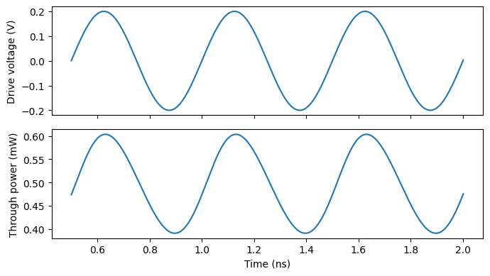
so our \(\mathrm{d}n / \mathrm{d}V = 5 \times 10^{-5}\) /V corresponds to \(V_{\pi L} = 1.55\) V·cm, representative of a depletion-mode silicon junction. Biasing the laser on the flank of the resonance, where the transmission slope is steepest, converts the resonance shift into intensity modulation: we bias half a linewidth above resonance and drive with a 0.2 V, 2 GHz sine from a signal_source. For the dynamics of microring modulators at frequencies comparable to the cavity linewidth, including the optical peaking effect, see the Microring Modulator Optical Peaking example.

dn_dv = 5e-5

# Bias the laser half a linewidth above resonance (maximum slope region)
f_laser = f_res + fwhm / 2
ring_eo = pfa.ring_resonator(
    kappa1=kappa,
    length=length,
    n_eff=n_eff_at(f_laser),
    reference_frequency=f_laser,
    n_group=n_group,
    propagation_loss=loss,
    dn_dv=dn_dv,
)

drive_freq = 2e9
source = pfa.signal_source(frequency=drive_freq, amplitude=0.2 / np.sqrt(z0))

# Laser and drive source connected to the ring, through port exposed
mrm = pf.Component("mrm_link")
laser_ref = mrm.add_reference(pfa.cw_laser(power=1e-3))
ring_ref = mrm.add_reference(ring_eo)
source_ref = mrm.add_reference(source)
ring_ref.connect("P0", laser_ref["P0"])
source_ref.connect("E0", ring_ref["E0"])
mrm.add_port(ring_ref["P1"], "out")
mrm.add_model(pf.CircuitModel(), "Circuit")

# A monitor on the electrical port records the voltage that drives the ring
num_steps = 100000
t = np.arange(num_steps) * time_step
time_stepper = mrm.setup_time_stepper(
    time_step=time_step,
    carrier_frequency=f_laser,
    time_stepper_kwargs={"monitors": {"drive": ring_ref["E0"]}},
)
output = time_stepper.step(steps=num_steps, time_step=time_step)
power = np.abs(output["out@0"]) ** 2 * 1e3
drive = np.real(output["drive@0-"]) * np.sqrt(z0)

# Plot the steady state, after the initial cavity charging transient
window = slice(25000, None)
fig, (ax1, ax2) = plt.subplots(2, 1, figsize=(7, 4), sharex=True, tight_layout=True)
ax1.plot(t[window] * 1e9, drive[window])
ax1.set_ylabel("Drive voltage (V)")
ax2.plot(t[window] * 1e9, power[window])
ax2.set(xlabel="Time (ns)", ylabel="Through power (mW)")

print(f"Resonance shift: {f_res * dn_dv / n_group / 1e9:.2f} GHz/V")

Resonance shift: 2.31 GHz/V

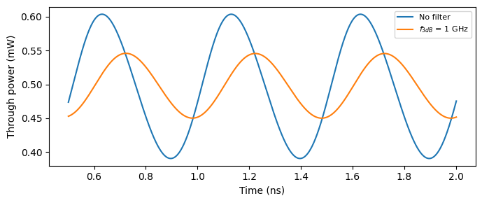
The f_3dB argument models the electrical bandwidth of the tuning port: a first-order low-pass filter applied directly to the input voltage, before it is converted to an index shift. With \(f_{3\mathrm{dB}} = 1\) GHz and the same 2 GHz drive, the voltage reaching the ring is attenuated by \(1 / \sqrt{1 + (f_m / f_{3\mathrm{dB}})^2} \approx 0.45\) (and delayed by the filter phase), which shows up directly in the modulation swing.

# Enable the electrical low-pass filter and rerun the same circuit
ring_eo.update(f_3dB=1e9)
time_stepper = mrm.setup_time_stepper(
    time_step=time_step, carrier_frequency=f_laser, show_progress=False
)
power_filtered = np.abs(
    time_stepper.step(steps=num_steps, time_step=time_step, show_progress=False)["out@0"]
) ** 2 * 1e3

fig, ax = plt.subplots(figsize=(7, 3), tight_layout=True)
ax.plot(t[window] * 1e9, power[window], label="No filter")
ax.plot(t[window] * 1e9, power_filtered[window], label="$f_{3dB}$ = 1 GHz")
ax.set(xlabel="Time (ns)", ylabel="Through power (mW)")
ax.legend(fontsize=8)

swing = power[window].max() - power[window].min()
swing_filtered = power_filtered[window].max() - power_filtered[window].min()
filter_response = 1 / np.sqrt(1 + (drive_freq / 1e9) ** 2)
print(f"Swing ratio: {swing_filtered / swing:.3f} "
      f"(first-order filter response at 2 GHz: {filter_response:.3f})")

Swing ratio: 0.450 (first-order filter response at 2 GHz: 0.447)

Summary

• pfa.ring_resonator models an all-pass ring with kappa1 or an add-drop ring with kappa1 and kappa2; ports map to input, through, drop, and add in sorted order, plus the electrical tuning port E0 (close it with an electrical_termination when unused).

• The coupler convention \(\tau = -i e^{i \arg \kappa} \sqrt{1 - \lvert \kappa \rvert^2}\) is shared with the frequency-domain RingModel, so time-domain and S-matrix results line up directly.

• The time stepper describes the ring at the carrier frequency: when the laser moves, update n_eff together with reference_frequency using \(n_\mathrm{eff}(f) = n_g + (n_\mathrm{eff}(f_\mathrm{ref}) - n_g) f_\mathrm{ref} / f\), and choose the time step as an integer fraction of the round-trip time.

• Cavity dynamics come out naturally: the charging transient decays with the field lifetime \(\tau = 1 / (\pi \, \mathrm{FWHM})\).

• dn_dT tunes the resonance thermally and dn_dv electro-optically, with \(\mathrm{d}n / \mathrm{d}V = \lambda_0 / (2 V_{\pi L})\) for a phase shifter specified by \(V_{\pi L}\); biasing on the resonance flank converts the shift into intensity modulation, the basis of the microring modulator.

• f_3dB applies a first-order low-pass filter directly to the input voltage, modeling the electrical bandwidth of the tuning port.