Signal Source

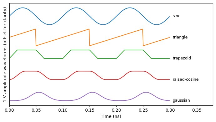
Modulators, switches, and tunable elements in a time-domain simulation all need electrical drive signals. The WaveformTimeStepper is PhotonForge’s signal generator: a single source that produces sine, triangle, trapezoid, raised-cosine, and Gaussian waveforms, gates them in time, encodes digital bit patterns (including pseudorandom bit sequences), and adds amplitude noise and clock jitter when a realistic drive is needed.

Like all electrical signals in the time-domain framework, the generated waveform is a real-valued wave amplitude in units of \(\sqrt{\mathrm{W}}\): a source set to produce a voltage \(V\) outputs the amplitude \(V / \sqrt{Z_0}\), and the voltage anywhere in a circuit is recovered as \(V = \Re \lbrace A \rbrace \sqrt{Z_0}\).

This guide tours the waveform library, time gating, digital patterns and eye diagrams, noise and jitter, and closes with the alternative to a signal source: injecting arbitrary user-defined signals directly into a circuit.

Setup

import matplotlib.pyplot as plt
import numpy as np
import photonforge as pf
import photonforge.abstract as pfa

viewer = pf.live_viewer.LiveViewer()

LiveViewer started at http://localhost:52135

tech = pf.basic_technology()
pf.config.default_technology = tech

lda0 = 1.55
f0 = pf.C_0 / lda0
z0 = 50.0
time_step = 1e-12

Waveform Library

The abstract signal_source component wraps the waveform time stepper in a single-port generator. Since it is a source, it can be simulated on its own: we initialize a time stepper directly on the component and read the generated signal from its electrical port E0.

The waveform argument selects the shape. Sine and triangle waves swing between offset - amplitude and offset + amplitude, while the pulsed shapes (trapezoid, raised-cosine, and Gaussian) are unipolar, ranging from offset to offset + amplitude. Pulse shapes are controlled in fractions of the source period: width sets the full width at half maximum, rise and fall set the edge times of trapezoid and raised-cosine pulses, skew sets the triangle asymmetry, and order turns the Gaussian into a flat-topped super-Gaussian.

source = pfa.signal_source(frequency=10e9, amplitude=1 / np.sqrt(z0))
viewer(source)

frequency = 10e9
num_steps = 300
t = np.arange(num_steps) * time_step

waveforms = {
    "sine": {},
    "triangle": {"skew": 1},
    "trapezoid": {"width": 0.5, "rise": 0.15, "fall": 0.15},
    "raised-cosine": {"width": 0.5, "rise": 0.3, "fall": 0.3},
    "gaussian": {"width": 0.35},
}

fig, ax = plt.subplots(figsize=(7, 4), tight_layout=True)
for k, (waveform, kwargs) in enumerate(waveforms.items()):
    source = pfa.signal_source(
        frequency=frequency, amplitude=1 / np.sqrt(z0), waveform=waveform, **kwargs
    )
    time_stepper = source.setup_time_stepper(
        time_step=time_step, carrier_frequency=f0, show_progress=False
    )
    output = time_stepper.step(steps=num_steps, time_step=time_step, show_progress=False)
    voltage = np.real(output["E0@0"]) * np.sqrt(z0)
    ax.plot(t * 1e9, voltage + 2.5 * (len(waveforms) - 1 - k))
    ax.text(0.305, 2.5 * (len(waveforms) - 1 - k), waveform, va="center", fontsize=9)

ax.set(xlabel="Time (ns)", xlim=(0, 0.38), yticks=[])
_ = ax.set_ylabel("1 V amplitude waveforms (offset for clarity)")

Time Gating

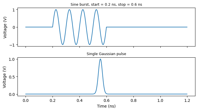
The start and stop arguments gate the source in time, which is useful for bursts, delayed drives, and settling experiments. A stopped source completes its current pulse before turning off, so the effective stop time can be slightly later than requested.

A single, isolated pulse is a common special case: gating one period of a pulsed waveform produces exactly one pulse, as in the Gaussian example below, often used to extract impulse responses.

num_steps = 1200
t = np.arange(num_steps) * time_step

sources = {
    "Sine burst, start = 0.2 ns, stop = 0.6 ns": pfa.signal_source(
        frequency=frequency, amplitude=1 / np.sqrt(z0), start=0.2e-9, stop=0.6e-9
    ),
    "Single Gaussian pulse": pfa.signal_source(
        frequency=frequency,
        amplitude=1 / np.sqrt(z0),
        waveform="gaussian",
        width=0.35,
        start=0.5e-9,
        stop=0.5e-9 + 1 / frequency,
    ),
}

fig, axes = plt.subplots(2, 1, figsize=(7, 4), sharex=True, tight_layout=True)
for ax, (label, source) in zip(axes, sources.items()):
    time_stepper = source.setup_time_stepper(
        time_step=time_step, carrier_frequency=f0, show_progress=False
    )
    output = time_stepper.step(steps=num_steps, time_step=time_step, show_progress=False)
    ax.plot(t * 1e9, np.real(output["E0@0"]) * np.sqrt(z0))
    ax.set_title(label, fontsize=9)
    ax.set_ylabel("Voltage (V)")
_ = axes[-1].set_xlabel("Time (ns)")

Digital Patterns

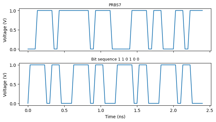
Setting prbs to 7, 15, or 31 turns the source into a pattern generator that emits the corresponding pseudorandom bit sequence at a bit rate given by frequency, using the selected waveform for pulse shaping. A user-defined pattern can be supplied through bit_sequence instead (with prbs=0), and it repeats indefinitely.

Trapezoid and raised-cosine shapes are the natural choices for digital signals. With those, width = 0.5 gives return-to-zero (RZ) coding, and width = 1 + 0.5 (rise + fall) gives non-return-to-zero (NRZ), where consecutive ones merge without dips. Below, a 10 Gb/s NRZ PRBS7 stream and a repeating user pattern, both with 30% rise and fall times.

bit_rate = 10e9
rise = fall = 0.3
nrz_width = 1 + 0.5 * (rise + fall)
unit_interval = int(round(1 / bit_rate / time_step))

patterns = {
    "PRBS7": {"prbs": 7, "seed": 0},
    "Bit sequence 1 1 0 1 0 0": {"bit_sequence": "110100"},
}

fig, axes = plt.subplots(2, 1, figsize=(7, 4), sharex=True, tight_layout=True)
for ax, (label, kwargs) in zip(axes, patterns.items()):
    source = pfa.signal_source(
        frequency=bit_rate,
        amplitude=1 / np.sqrt(z0),
        waveform="trapezoid",
        rise=rise,
        fall=fall,
        width=nrz_width,
        **kwargs,
    )
    time_stepper = source.setup_time_stepper(
        time_step=time_step, carrier_frequency=f0, show_progress=False
    )
    num_steps = unit_interval * 24
    t = np.arange(num_steps) * time_step
    output = time_stepper.step(steps=num_steps, time_step=time_step, show_progress=False)
    ax.plot(t * 1e9, np.real(output["E0@0"]) * np.sqrt(z0))
    ax.set_title(label, fontsize=9)
    ax.set_ylabel("Voltage (V)")
_ = axes[-1].set_xlabel("Time (ns)")

Noise, Jitter, and Eye Diagrams

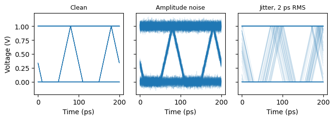
Real drivers are not ideal: noise adds white amplitude noise with the given one-sided amplitude spectral density (in \(\sqrt{\mathrm{W} / \mathrm{Hz}}\), so the resulting variance depends on the simulation bandwidth \(1 / (2 \Delta t)\)), and jitter displaces the pattern edges with the given RMS clock jitter. Since jitter is simulated in whole time steps, the time step should be well below the jitter value for an accurate representation; here we use a 0.25 ps step for 2 ps of jitter.

Folding a long pattern into segments of two unit intervals produces the eye diagram, the standard way to judge signal quality. Comparing the clean source with one adding \(4 \times 10^{-9}\) \(\sqrt{\mathrm{W} / \mathrm{Hz}}\) of amplitude noise and one with 2 ps RMS jitter shows the eye closing vertically with noise and horizontally with jitter.

time_step_eye = 0.25e-12
unit_interval = int(round(1 / bit_rate / time_step_eye))
num_bits = 256
num_steps = unit_interval * num_bits
t_eye = np.arange(2 * unit_interval) * time_step_eye

cases = {
    "Clean": {},
    "Amplitude noise": {"noise": 4e-9},
    "Jitter, 2 ps RMS": {"jitter": 2e-12},
}

fig, axes = plt.subplots(1, 3, figsize=(7, 2.6), sharey=True, tight_layout=True)
for ax, (label, kwargs) in zip(axes, cases.items()):
    source = pfa.signal_source(
        frequency=bit_rate,
        amplitude=1 / np.sqrt(z0),
        waveform="trapezoid",
        rise=rise,
        fall=fall,
        width=nrz_width,
        prbs=7,
        seed=0,
        **kwargs,
    )
    time_stepper = source.setup_time_stepper(
        time_step=time_step_eye, carrier_frequency=f0, show_progress=False
    )
    output = time_stepper.step(steps=num_steps, time_step=time_step_eye, show_progress=False)
    voltage = np.real(output["E0@0"]) * np.sqrt(z0)
    segments = voltage[unit_interval // 2 :]
    segments = segments[: len(segments) // (2 * unit_interval) * 2 * unit_interval]
    for segment in segments.reshape(-1, 2 * unit_interval):
        ax.plot(t_eye * 1e12, segment, color="C0", alpha=0.15, linewidth=0.8)
    ax.set_title(label, fontsize=9)
    ax.set_xlabel("Time (ps)")
axes[0].set_ylabel("Voltage (V)")
plt.show()

Injecting Arbitrary Signals

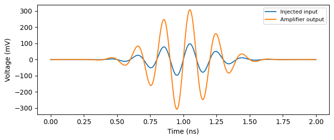
The signal source covers the common cases, but any waveform can be injected directly. The step method accepts a TimeSeries of input samples keyed by port names, so a signal computed in Python (or loaded from a measurement) drives a component or circuit without any source component.

As a minimal example, we feed a Gaussian-windowed sine burst into an electrical_amplifier with 10 dB of gain, running the time stepper directly on the component and keying the input by its own port, E0. When inputs is given, the number of steps and time step come from the time series itself.

amplifier = pfa.electrical_amplifier(gain=10)

num_steps = 2000
t = np.arange(num_steps) * time_step
v_in = 0.1 * np.sin(2 * np.pi * 5e9 * t) * np.exp(-(((t - 1e-9) / 0.3e-9) ** 2))

inputs = pf.TimeSeries({"E0@0": v_in / np.sqrt(z0)}, time_step)
time_stepper = amplifier.setup_time_stepper(time_step=time_step, carrier_frequency=f0)
output = time_stepper.step(inputs=inputs)
v_out = np.real(output["E1@0"]) * np.sqrt(z0)

fig, ax = plt.subplots(figsize=(7, 3), tight_layout=True)
ax.plot(t * 1e9, v_in * 1e3, label="Injected input")
ax.plot(t * 1e9, v_out * 1e3, label="Amplifier output")
ax.set(xlabel="Time (ns)", ylabel="Voltage (mV)")
_ = ax.legend(fontsize=8)

Summary

• pfa.signal_source is the electrical signal generator for time-domain simulations, producing sine, triangle, trapezoid, raised-cosine, and Gaussian waveforms with amplitudes specified as \(V / \sqrt{Z_0}\).

• Pulse shapes are parametrized as fractions of the period (width, rise, fall, skew, order), and start / stop gate the source in time, down to a single isolated pulse.

• prbs or bit_sequence generate digital patterns at a bit rate set by frequency; with trapezoid or raised-cosine shaping, width = 0.5 gives RZ and width = 1 + 0.5 (rise + fall) gives NRZ coding.

• noise (amplitude spectral density) and jitter (RMS) model driver imperfections, closing the eye diagram vertically and horizontally; seed makes realizations reproducible.

• Arbitrary waveforms can bypass the source entirely: pass a TimeSeries keyed by port names to step to inject any signal directly into a component or circuit.

• This source drives the modulators shown in the other guides of this section, and the optical counterpart sources are described by the CWLaserTimeStepper and OpticalPulseTimeStepper.