

Bayesian optimization of a SOI vertical grating coupler#
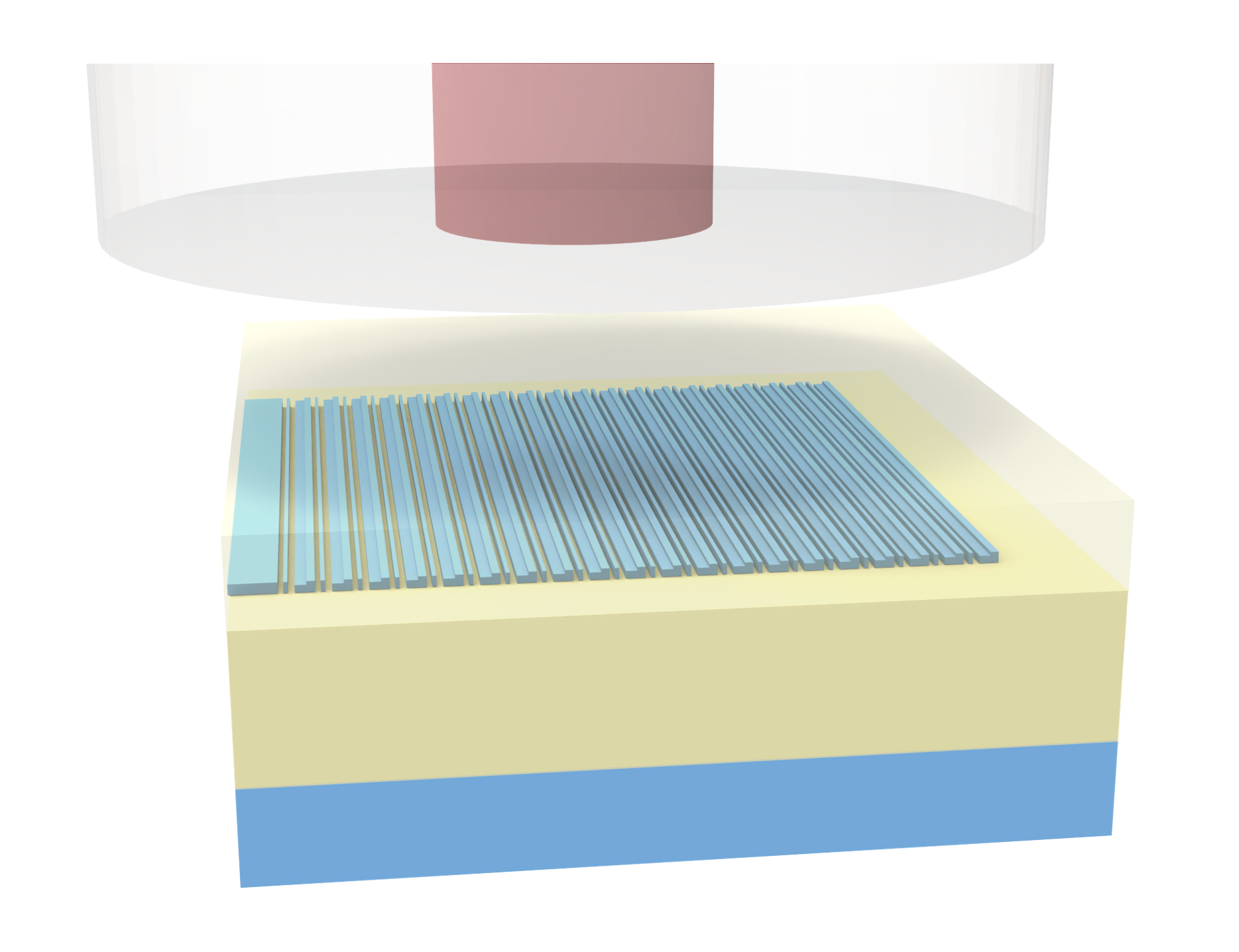
Grating couplers are photonic devices that couple light efficiently between optical fibers and integrated photonic waveguides. They work by diffracting light incident from above into the plane of the chip, enabling vertical fiber-to-chip coupling—a key functionality for scalable photonic integrated circuits. Vertical grating couplers are widely used because they simplify packaging and alignment compared to edge coupling, and can be designed with high efficiency for target wavelengths, such as the telecom band around 1.55 μm.
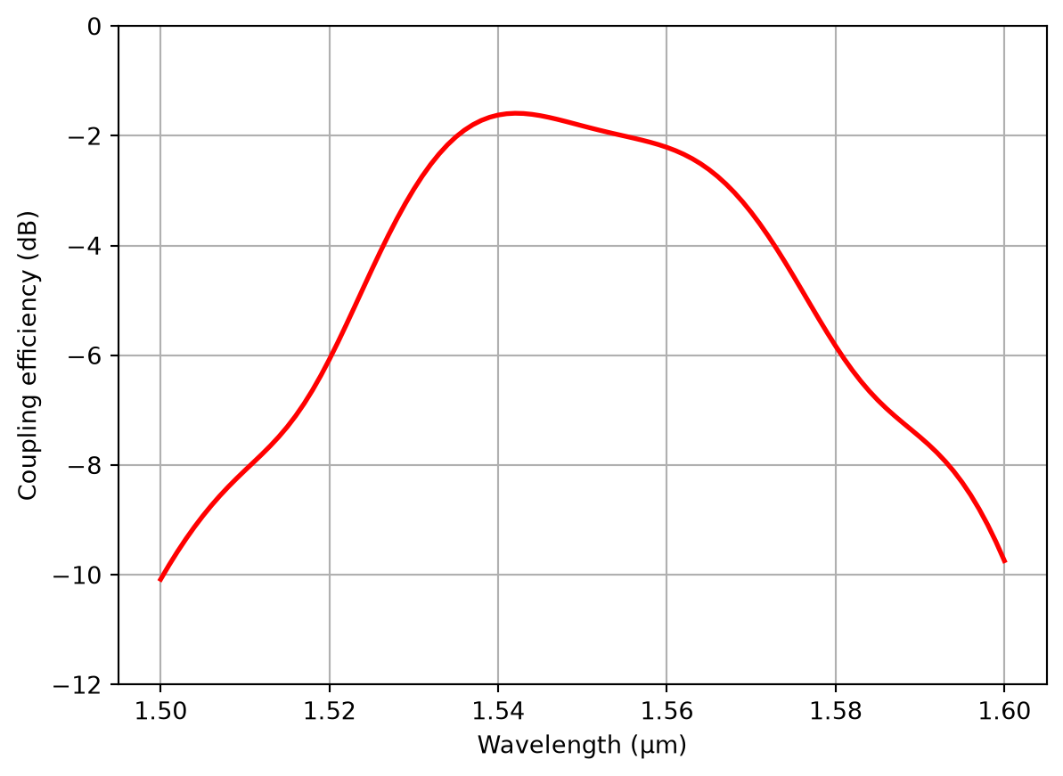
This notebook demonstrates the design optimization of a vertical grating coupler using the Bayesian optimizer from Tidy3D’s design plugin. The optimized design achieves a < 2dB coupling efficiency. The design is based on the work T. Watanabe, M. Ayata, U. Koch, Y. Fedoryshyn and J. Leuthold, "Perpendicular Grating Coupler Based on a Blazed Antiback-Reflection Structure," in Journal of Lightwave Technology, vol. 35, no. 21, pp. 4663-4669, 1 Nov.1, 2017. DOI:
10.1109/JLT.2017.2755673.
[1]:
# Standard library imports
import matplotlib.pyplot as plt
import numpy as np

# Tidy3D imports
import tidy3d as td
import tidy3d.plugins.design as tdd
import tidy3d.web as web
Simulation Setup#
We define the simulation parameters, including the wavelength range, fixed geometric parameters, and the materials (silicon and silicon oxide).
[2]:
# Define frequency and wavelength range
lda0 = 1.55  # Central wavelength
freq0 = td.C_0 / lda0  # Central frequency
ldas = np.linspace(1.5, 1.6, 101)  # Wavelength range
freqs = td.C_0 / ldas  # Frequency range
fwidth = 0.5 * (np.max(freqs) - np.min(freqs))  # Frequency width of the source
[3]:
# Geometric parameters
h_si = 0.22  # Silicon thickness
h_etch = 0.07  # Etch depth
h_box = 3  # Buried oxide thickness
h_clad = 1.5  # Cladding thickness
n = 20  # Number of grating periods
mfd = 10.4  # Mode field diameter
ly = 15  # Grating size in y

# Materials
n_si = 3.45
mat_si = td.Medium(permittivity=n_si**2)

n_sio2 = 1.45
mat_sio2 = td.Medium(permittivity=n_sio2**2)
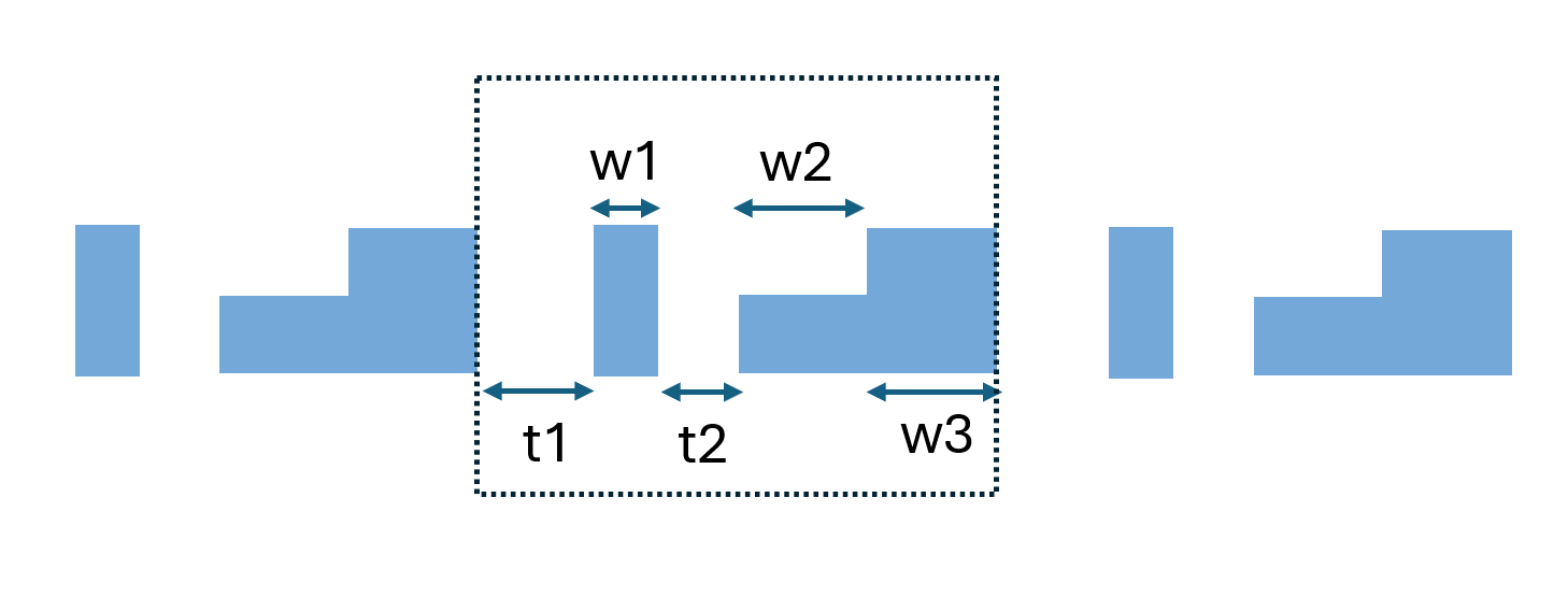
The grating coupler geometry is parameterized by the thickness and width of the grating teeth (t1, t2, w1, w2, w3). The make_grating function constructs the grating geometry, and make_sim_2d creates the full Tidy3D simulation, including the waveguide, substrate, source, and monitors. We will start our optimization in 2D since it’s much faster and cheaper. Then we will verify the optimal design with the full 3D simulation.
[4]:
def make_grating(t1, t2, w1, w2, w3):
    """Constructs the grating geometry based on parameters."""
    p = t1 + t2 + w1 + w2 + w3  # Grating period
    grating = 0
    for i in range(n):
        # First tooth section
        grating += td.Box.from_bounds(
            rmin=(i * p + t1, -ly / 2, 0), rmax=(i * p + t1 + w1, ly / 2, h_si)
        )

        # Etched section
        grating += td.Box.from_bounds(
            rmin=(i * p + t1 + w1 + t2, -ly / 2, 0),
            rmax=(i * p + t1 + w1 + t2 + w2, ly / 2, h_si - h_etch),
        )

        # Second tooth section
        grating += td.Box.from_bounds(
            rmin=(i * p + t1 + w1 + t2 + w2, -ly / 2, 0),
            rmax=(i * p + t1 + w1 + t2 + w2 + w3, ly / 2, h_si),
        )

    return td.Structure(geometry=grating, medium=mat_si)
[5]:
def make_sim_2d(t1, t2, w1, w2, w3):
    """Creates the Tidy3D simulation."""
    grating = make_grating(t1, t2, w1, w2, w3)

    p = t1 + t2 + w1 + w2 + w3  # Grating period
    lx = p * n  # Grating size in x
    inf_eff = 1e3  # effective infinity

    # Waveguide
    waveguide = td.Structure(
        geometry=td.Box.from_bounds(rmin=(-inf_eff, -ly / 2, 0), rmax=(0, ly / 2, h_si)),
        medium=mat_si,
    )

    # Cladding and buried oxide
    box_clad = td.Structure(
        geometry=td.Box.from_bounds(
            rmin=(-inf_eff, -inf_eff, -h_box), rmax=(inf_eff, inf_eff, h_clad + h_si)
        ),
        medium=mat_sio2,
    )

    # Substrate
    substrate = td.Structure(
        geometry=td.Box.from_bounds(
            rmin=(-inf_eff, -inf_eff, -h_box - inf_eff), rmax=(inf_eff, inf_eff, -h_box)
        ),
        medium=mat_si,
    )

    # Gaussian beam source
    gaussian_beam = td.GaussianBeam(
        center=(lx / 2, 0, h_clad + lda0 / 2),
        size=(2 * mfd, 2 * mfd, 0),
        source_time=td.GaussianPulse(freq0=freq0, fwidth=fwidth),
        pol_angle=np.pi / 2,
        angle_theta=0,
        angle_phi=0,
        direction="-",
        waist_radius=mfd / 2,
        waist_distance=0,
    )

    # Mode monitor
    mode_monitor = td.ModeMonitor(
        center=(-lda0 / 2, 0, h_si / 2),
        size=(0, 1.5 * ly, 5 * h_si),
        freqs=freqs,
        mode_spec=td.ModeSpec(num_modes=1, target_neff=n_si),
        name="mode",
    )

    # Simulation domain box
    sim_box = td.Box.from_bounds(
        rmin=(-0.6 * lda0, 0, -h_box - 0.6 * lda0),
        rmax=(lx + 0.6 * lda0, 0, h_clad + h_si + 0.6 * lda0),
    )

    # Define the simulation
    sim = td.Simulation(
        center=sim_box.center,
        size=sim_box.size,
        grid_spec=td.GridSpec.auto(min_steps_per_wvl=20),
        run_time=1e-11,
        structures=[substrate, box_clad, grating, waveguide],
        sources=[gaussian_beam],
        monitors=[mode_monitor],
        boundary_spec=td.BoundarySpec(
            x=td.Boundary.pml(),
            y=td.Boundary.periodic(),  # set the boundary to periodic in y since it's a 2D simulation
            z=td.Boundary.pml(),
        ),
    )
    return sim
[6]:
# Create a simulation instance with some arbitrary parameters
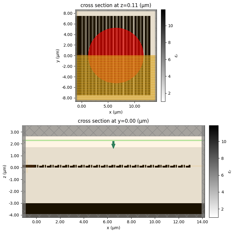
sim = make_sim_2d(t1=0.1, t2=0.1, w1=0.1, w2=0.25, w3=0.1)

# Visualize the permittivity distribution
sim.plot_eps(y=0)
plt.show()
Optimization#
Bayesian optimization is a powerful strategy for optimizing expensive-to-evaluate functions, using a probabilistic model to efficiently explore the parameter space and identify optimal solutions with fewer simulations.
To optimize the grating design for maximal coupling efficiency at 1550 nm, we configure the Bayesian optimization using MethodBayOpt.
We define the design space for the grating parameters and specify the objective function compute_transmission, which calculates the transmission efficiency based on the mode monitor data.
[7]:
def compute_transmission(sim_data):
    """Calculates the coupling efficiency from the simulation data."""
    # Extract mode amplitude data at 1550 nm
    T = np.abs(sim_data["mode"].amps.sel(mode_index=0, f=freq0, direction="-").values) ** 2
    # Return coupling efficiency in dB
    return 10 * np.log10(T)
To ensure fabrication constraint, we limit the minimal feature size to 50 nm. All design parameters have a range from 50 nm to 250 nm.
After running the optimization, we achieved a design with sub 2dB coupling efficiency.
[8]:
# Define optimization method (Bayesian optimization)
method = tdd.MethodBayOpt(
    initial_iter=50,
    n_iter=150,
    acq_func="ucb",
    kappa=1,
    seed=4,
)

span = (0.05, 0.25)  # Parameter value range

# Define optimization parameters
parameters = [
    tdd.ParameterFloat(name="t1", span=span),
    tdd.ParameterFloat(name="t2", span=span),
    tdd.ParameterFloat(name="w1", span=span),
    tdd.ParameterFloat(name="w2", span=span),
    tdd.ParameterFloat(name="w3", span=span),
]

# Define a design space
design_space = tdd.DesignSpace(
    method=method, parameters=parameters, task_name="bay_opt", path_dir="./data"
)

# Run the design optimization
results = design_space.run(make_sim_2d, compute_transmission, verbose=True)
14:23:27 UTC Running 50 Simulations
14:24:29 UTC Best Fit from Initial Solutions: -7.699
Running 1 Simulations
14:24:32 UTC Running 1 Simulations
14:24:36 UTC Running 1 Simulations
14:24:39 UTC Running 1 Simulations
14:24:43 UTC Running 1 Simulations
14:24:48 UTC Running 1 Simulations
14:24:52 UTC Running 1 Simulations
14:24:55 UTC Running 1 Simulations
14:24:58 UTC Latest Best Fit on Iter 7: -7.638
14:24:59 UTC Running 1 Simulations
14:25:02 UTC Running 1 Simulations
14:25:06 UTC Latest Best Fit on Iter 9: -6.465
Running 1 Simulations
14:25:09 UTC Running 1 Simulations
14:25:13 UTC Latest Best Fit on Iter 11: -6.084
Running 1 Simulations
14:25:17 UTC Running 1 Simulations
14:25:20 UTC Running 1 Simulations
14:25:24 UTC Latest Best Fit on Iter 14: -5.192
Running 1 Simulations
14:25:27 UTC Latest Best Fit on Iter 15: -4.784
Running 1 Simulations
14:25:31 UTC Running 1 Simulations
14:25:34 UTC Running 1 Simulations
14:25:37 UTC Running 1 Simulations
14:25:41 UTC Running 1 Simulations
14:25:44 UTC Running 1 Simulations
14:25:48 UTC Running 1 Simulations
14:25:52 UTC Running 1 Simulations
14:25:55 UTC Latest Best Fit on Iter 23: -2.823
Running 1 Simulations
14:25:59 UTC Running 1 Simulations
14:26:02 UTC Running 1 Simulations
14:26:06 UTC Running 1 Simulations
14:26:09 UTC Running 1 Simulations
14:26:13 UTC Running 1 Simulations
14:26:16 UTC Running 1 Simulations
14:26:20 UTC Running 1 Simulations
14:26:23 UTC Running 1 Simulations
14:26:27 UTC Running 1 Simulations
14:26:40 UTC Running 1 Simulations
14:26:44 UTC Running 1 Simulations
14:26:48 UTC Latest Best Fit on Iter 35: -2.496
Running 1 Simulations
14:26:51 UTC Latest Best Fit on Iter 36: -2.38
14:26:52 UTC Running 1 Simulations
14:26:55 UTC Running 1 Simulations
14:26:59 UTC Running 1 Simulations
14:27:02 UTC Latest Best Fit on Iter 39: -2.285
Running 1 Simulations
14:27:06 UTC Latest Best Fit on Iter 40: -2.236
Running 1 Simulations
14:27:10 UTC Running 1 Simulations
14:27:13 UTC Running 1 Simulations
14:27:17 UTC Latest Best Fit on Iter 43: -2.174
Running 1 Simulations
14:27:21 UTC Running 1 Simulations
14:27:24 UTC Running 1 Simulations
14:27:28 UTC Running 1 Simulations
14:27:31 UTC Running 1 Simulations
14:27:35 UTC Running 1 Simulations
14:27:38 UTC Running 1 Simulations
14:27:43 UTC Running 1 Simulations
14:27:46 UTC Latest Best Fit on Iter 51: -2.084
Running 1 Simulations
14:27:49 UTC Latest Best Fit on Iter 52: -2.003
14:27:50 UTC Running 1 Simulations
14:27:53 UTC Running 1 Simulations
14:27:56 UTC Running 1 Simulations
14:28:00 UTC Running 1 Simulations
14:28:03 UTC Running 1 Simulations
14:28:07 UTC Latest Best Fit on Iter 57: -1.94
Running 1 Simulations
14:28:11 UTC Running 1 Simulations
14:28:14 UTC Running 1 Simulations
14:28:18 UTC Running 1 Simulations
14:28:21 UTC Running 1 Simulations
14:28:25 UTC Running 1 Simulations
14:28:28 UTC Running 1 Simulations
14:28:32 UTC Running 1 Simulations
14:28:35 UTC Running 1 Simulations
14:28:38 UTC Running 1 Simulations
14:28:42 UTC Running 1 Simulations
14:28:45 UTC Running 1 Simulations
14:28:49 UTC Running 1 Simulations
14:28:52 UTC Running 1 Simulations
14:28:56 UTC Running 1 Simulations
14:28:59 UTC Running 1 Simulations
14:29:03 UTC Running 1 Simulations
14:29:06 UTC Running 1 Simulations
14:29:10 UTC Running 1 Simulations
14:29:13 UTC Running 1 Simulations
14:29:17 UTC Running 1 Simulations
14:29:21 UTC Running 1 Simulations
14:29:24 UTC Running 1 Simulations
14:29:27 UTC Running 1 Simulations
14:29:31 UTC Running 1 Simulations
14:29:34 UTC Running 1 Simulations
14:29:38 UTC Running 1 Simulations
14:29:42 UTC Running 1 Simulations
14:29:45 UTC Running 1 Simulations
14:29:49 UTC Running 1 Simulations
14:29:52 UTC Running 1 Simulations
14:29:56 UTC Running 1 Simulations
14:30:00 UTC Running 1 Simulations
14:30:03 UTC Running 1 Simulations
14:30:07 UTC Running 1 Simulations
14:30:10 UTC Running 1 Simulations
14:30:14 UTC Running 1 Simulations
14:30:18 UTC Running 1 Simulations
14:30:21 UTC Running 1 Simulations
14:30:25 UTC Running 1 Simulations
14:30:29 UTC Running 1 Simulations
14:30:32 UTC Running 1 Simulations
14:30:36 UTC Running 1 Simulations
14:30:39 UTC Running 1 Simulations
14:30:44 UTC Running 1 Simulations
14:30:47 UTC Running 1 Simulations
14:30:51 UTC Running 1 Simulations
14:30:54 UTC Running 1 Simulations
14:30:58 UTC Running 1 Simulations
14:31:02 UTC Running 1 Simulations
14:31:06 UTC Running 1 Simulations
14:31:09 UTC Running 1 Simulations
14:31:13 UTC Running 1 Simulations
14:31:16 UTC Running 1 Simulations
14:31:20 UTC Running 1 Simulations
14:31:24 UTC Running 1 Simulations
14:31:27 UTC Running 1 Simulations
14:31:31 UTC Running 1 Simulations
14:31:34 UTC Running 1 Simulations
14:31:38 UTC Running 1 Simulations
14:31:41 UTC Running 1 Simulations
14:31:45 UTC Running 1 Simulations
14:31:48 UTC Running 1 Simulations
14:31:52 UTC Running 1 Simulations
14:31:55 UTC Running 1 Simulations
14:31:59 UTC Running 1 Simulations
14:32:02 UTC Running 1 Simulations
14:32:06 UTC Running 1 Simulations
14:32:09 UTC Latest Best Fit on Iter 125: -1.826
14:32:10 UTC Running 1 Simulations
14:32:13 UTC Running 1 Simulations
14:32:17 UTC Running 1 Simulations
14:32:21 UTC Running 1 Simulations
14:32:24 UTC Running 1 Simulations
14:32:28 UTC Latest Best Fit on Iter 130: -1.759
Running 1 Simulations
14:32:32 UTC Running 1 Simulations
14:32:35 UTC Running 1 Simulations
14:32:39 UTC Running 1 Simulations
14:32:42 UTC Running 1 Simulations
14:32:46 UTC Running 1 Simulations
14:32:49 UTC Running 1 Simulations
14:32:54 UTC Running 1 Simulations
14:32:57 UTC Running 1 Simulations
14:33:01 UTC Running 1 Simulations
14:33:05 UTC Running 1 Simulations
14:33:08 UTC Running 1 Simulations
14:33:12 UTC Running 1 Simulations
14:33:15 UTC Running 1 Simulations
14:33:19 UTC Running 1 Simulations
14:33:22 UTC Running 1 Simulations
14:33:26 UTC Running 1 Simulations
14:33:29 UTC Running 1 Simulations
14:33:33 UTC Running 1 Simulations
14:33:36 UTC Best Result: -1.759101800459121
             Best Parameters: t1: 0.05 t2: 0.05884944980504611 w1:
             0.1015323031540251 w2: 0.24139555731212883 w3: 0.17599800331530713
Final Design#
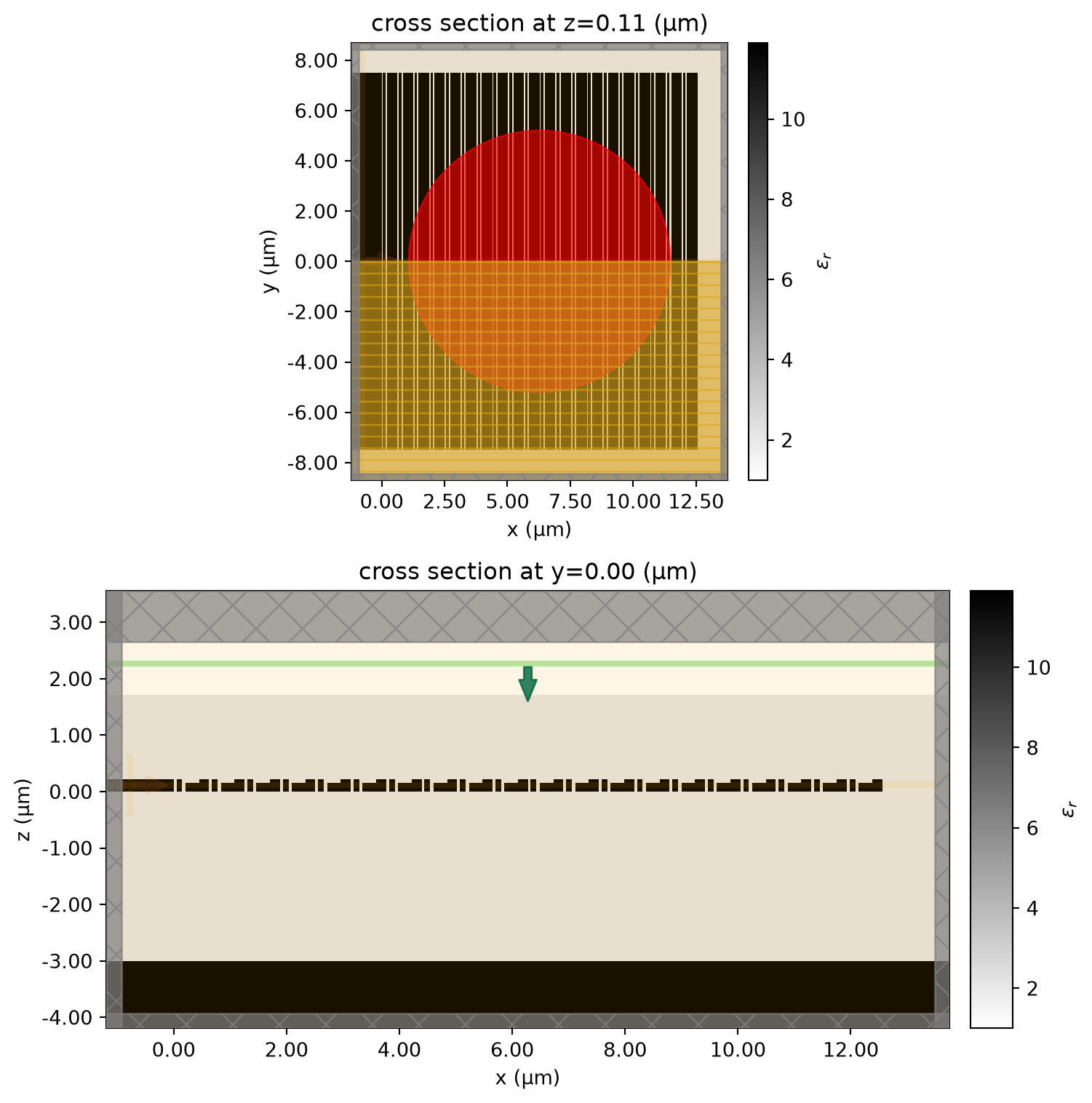
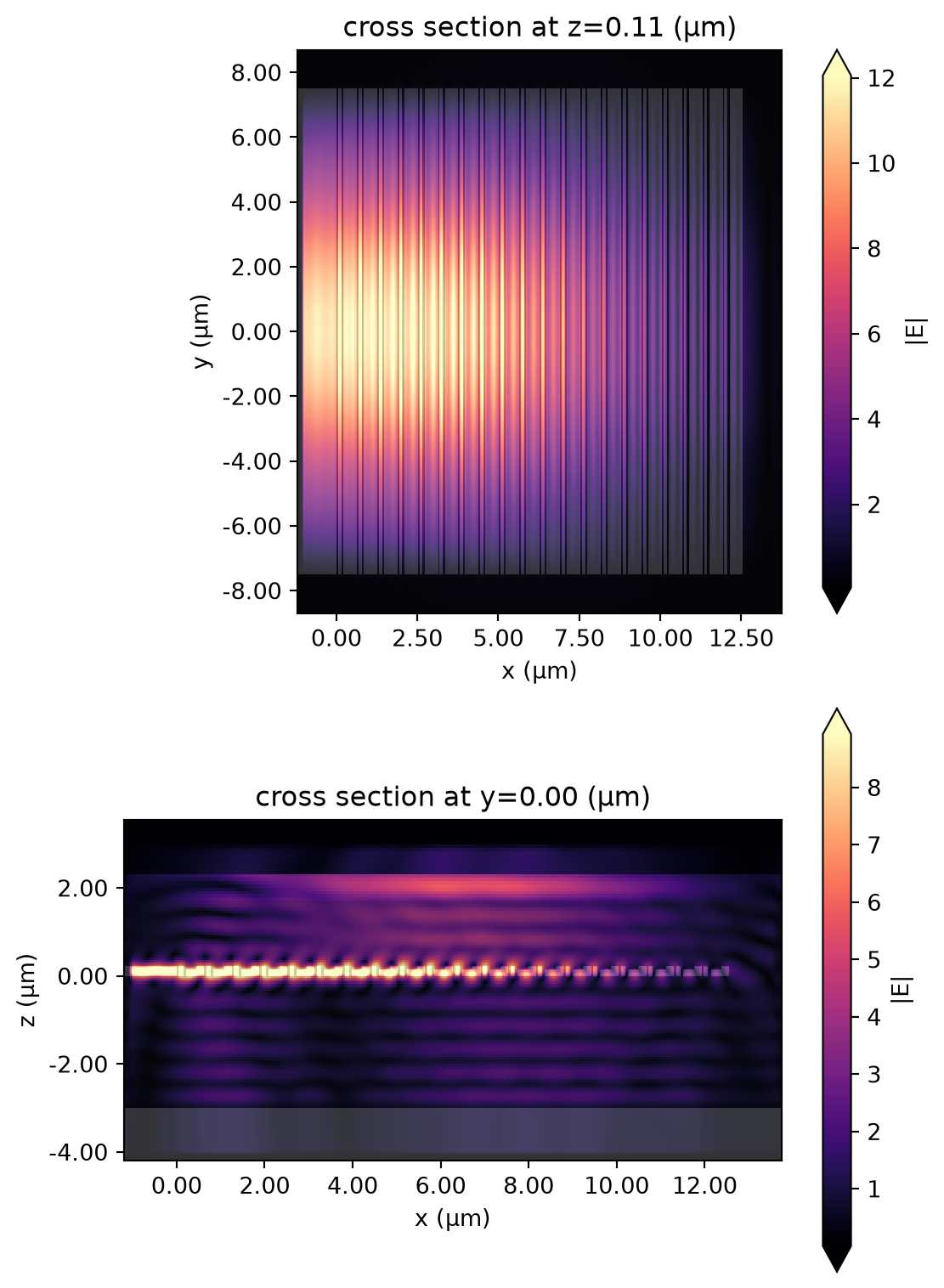
After the optimization runs, we extract the best parameters and then run a 3D final simulation with these optimal parameters to verify the design from the previous 2D simulations. The 3D simulation can be made by copying the 2D simulation and updating the simulation domain size and boundary condition. To help with visualization, we also added two FieldMonitors in the \(xy\) and \(xz\) planes. Also note that the 3D simulation has a symmetry in the \(y\) direction that we can utilize to reduce the computational cost and time.
[9]:
# Define field monitors for visualization
field_xy = td.FieldMonitor(
    center=(0, 0, h_si / 2), size=(td.inf, td.inf, 0), freqs=[freq0], name="field_xy"
)

field_xz = td.FieldMonitor(
    center=(0, 0, 0), size=(td.inf, 0, td.inf), freqs=[freq0], name="field_xz"
)

# Extract optimal parameters from the results
optimal_params = results.optimizer.max["params"]

# Make a 2D simulation with the optimal parameters
sim_opt = make_sim_2d(**optimal_params)

# Update simulation with monitors and new domain size to make it 3D
sim_opt = sim_opt.updated_copy(
    size=(sim_opt.size[0], ly + 1.2 * lda0, sim_opt.size[2]),
    monitors=[sim_opt.monitors[0], field_xy, field_xz],
    boundary_spec=td.BoundarySpec.all_sides(boundary=td.PML()),
    symmetry=(0, -1, 0),
)

# Plot the permittivity distribution of the optimal design
fig, ax = plt.subplots(2, 1, figsize=(8, 8), tight_layout=True)

# Plot the permittivity distribution in the xy plane
sim_opt.plot_eps(z=h_si / 2, ax=ax[0], monitor_alpha=0.1)

# Add a circle to indicate the mode field diameter
lx = sum(optimal_params.values()) * n
circle = plt.Circle((lx / 2, 0), mfd / 2, color="red", alpha=0.6, fill=True)
ax[0].add_patch(circle)

# Plot the permittivity distribution in the xz plane
sim_opt.plot_eps(y=0, ax=ax[1], monitor_alpha=0.1)
plt.show()
Run the 3D simulation and plot the coupling efficiency spectrum.
[10]:
# Run the 3D simulation
sim_data_opt = web.run(sim_opt, "optimal design")

# extract coupling efficiency and plot it
amp = sim_data_opt["mode"].amps.sel(mode_index=0, direction="-")
T = np.abs(amp) ** 2
plt.plot(ldas, 10 * np.log10(T), c="red", linewidth=2)
plt.ylim(-12, 0)
plt.xlabel("Wavelength (μm)")
plt.ylabel("Coupling efficiency (dB)")
plt.grid()
plt.show()
14:33:37 UTC Created task 'optimal design' with resource_id
             'fdve-a1b05b7d-388b-40be-84cb-5f3d394bf317' and task_type 'FDTD'.
             View task using web UI at
             'https://tidy3d.simulation.cloud/workbench?taskId=fdve-a1b05b7d-388
             b-40be-84cb-5f3d394bf317'.
Task folder: 'default'.
14:33:38 UTC Estimated FlexCredit cost: 3.649. This assumes the FDTD solver runs
             for the full simulation time; if early shutoff is reached, the
             billed cost can be lower. Use 'web.real_cost(task_id)' to get the
             billed FlexCredit cost after a simulation run.
14:33:39 UTC status = success
14:33:41 UTC Loading results from simulation_data.hdf5
Finally, plot the field distribution to visualize the mode coupling.
[11]:
fig, ax = plt.subplots(2, 1, figsize=(6, 8), tight_layout=True)
sim_data_opt.plot_field("field_xy", "E", "abs", ax=ax[0])
sim_data_opt.plot_field("field_xz", "E", "abs", ax=ax[1])
plt.show()
Final Notes#
The grating coupler is typically connected to a waveguide taper, which enables an adiabatic transition into a single-mode waveguide. In our simulation, we omit the taper to reduce computational cost. The taper itself can be optimized independently to ensure minimal loss, thereby maintaining a high overall coupling efficiency for the complete device.
In addition to Bayesian optimization, alternative optimization strategies, such as particle swarm optimization (PSO) and adjoint-based inverse design, can also be used to further improve device performance, for example through apodization.