Design optimization of a bilayer SiN/Si grating coupler

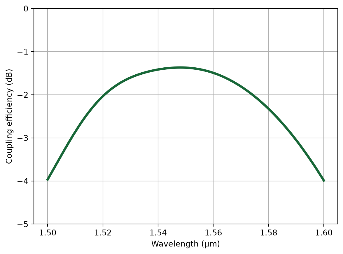
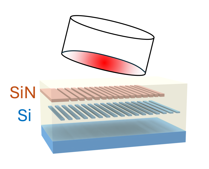
Silicon nitride has attracted increasing interest due to its superior passive properties. However, similar to silicon PICs, fiber-to-chip coupling remains a significant challenge for SiN platforms. Conventional SiN grating couplers exhibit low coupling efficiency due to their low refractive index contrast. To address this, a high-contrast grating reflector (GR) is employed as a bottom reflector to enhance coupling efficiency, rather than using distributed Bragg reflectors (DBR) or metal reflectors. Through design optimization, combining parameter sweeps and adjoint-based inverse design, a grating coupler with high coupling efficiency (< 1 dB) is achieved.

The workflow includes:

1. Periodic SiN Grating Coupler Design: Optimizing the SiN grating period, gap size, and fiber position.

2. Silicon Grating Reflector Design: Designing a bottom silicon grating to reflect leakage light upwards.

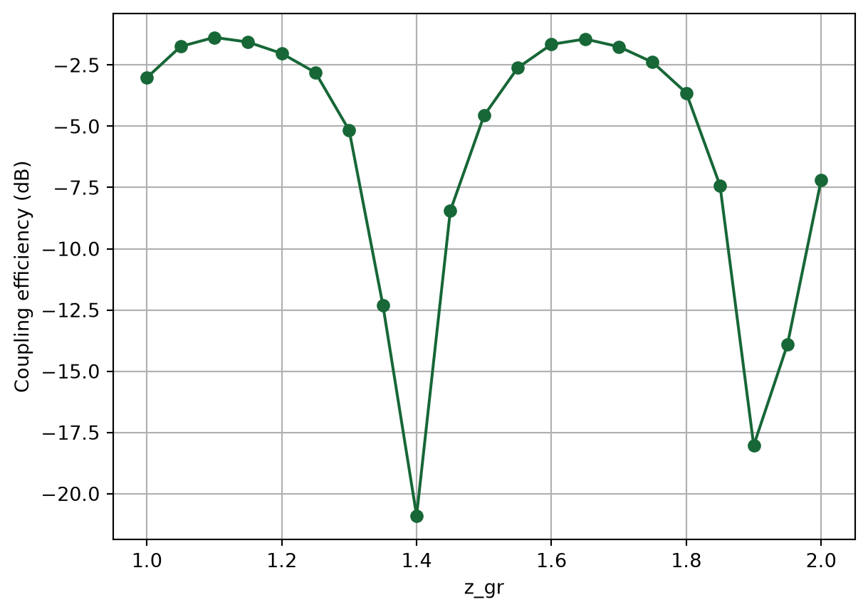
3. Interlayer Distance Optimization: Tuning the distance between the SiN and Si layers.

4. Inverse Design: Using adjoint optimization to apodize the grating for maximum efficiency.

The design is based on the following publication: Jinghui Zou, Yu Yu, Mengyuan Ye, Lei Liu, Shupeng Deng, and Xinliang Zhang, "Ultra efficient silicon nitride grating coupler with bottom grating reflector," Opt. Express 23, 26305-26312 (2015). DOI: 10.1364/OE.23.026305.

import autograd as ag
import autograd.numpy as np
import matplotlib.pyplot as plt
import tidy3d as td
import tidy3d.plugins.design as tdd
import tidy3d.web as web
from tidy3d.plugins.autograd import adam, apply_updates

Simulation Setup

We define the central wavelength, frequency, and bandwidth for the simulation. The simulation will target 1550 nm.

lda0 = 1.55  # Central wavelength
freq0 = td.C_0 / lda0  # Central frequency
ldas = np.linspace(1.5, 1.6, 101)  # Wavelength range
freqs = td.C_0 / ldas
fwidth = 0.5 * (np.max(freqs) - np.min(freqs))  # Frequency width of the source

We define the relevant materials as nondispersive mediums for simplicity.

SiN = td.Medium.from_nk(n=1.97, k=0, freq=freq0)
Si = td.Medium.from_nk(n=3.47, k=0, freq=freq0)
SiO2 = td.Medium.from_nk(n=1.44, k=0, freq=freq0)

Defining the fixed geometric parameters.

t_SiN = 0.4  # Thickness of SiN layer
t_Si = 0.22  # Thickness of Silicon waveguide
t_clad = 0.75  # Target cladding thickness
t_box = 2  # Thickness of Buried Oxide (BOX)
theta = np.deg2rad(8)  # Fiber angle
mfd = 10.4  # Mode field diameter

n_gc = 14  # Number of SiN grating teeth
inf_eff = 1e3  # Effective infinity

Next we define some fixed simulation parameters. These will be used repeatedly in various following simulation setups.

run_time = 3e-12  # Simulation run time

# Grid specification
grid_spec = td.GridSpec.auto(min_steps_per_wvl=20)

# Boundary condition specification
boundary_spec = td.BoundarySpec(
    x=td.Boundary.absorber(num_layers=80),
    y=td.Boundary.periodic(),  # set the boundary to periodic in y since it's a 2D simulation
    z=td.Boundary.pml(),
)

# Mode monitor for coupling efficiency measurement
mode_monitor = td.ModeMonitor(
    center=(-lda0 / 2, 0, t_SiN / 2),
    size=(0, td.inf, 5 * t_SiN),
    freqs=freqs,
    mode_spec=td.ModeSpec(num_modes=1, target_neff=1.97),
    name="mode",
)

Periodic SiN Grating Coupler Design

In the first part, we design and optimize a periodic SiN grating coupler by parameter sweeping the grating period, duty cycle, and fiber position.

Since we are optimizing the grating only, we will ignore the silicon layer as well as the substrate for now. They will be added and optimized later.

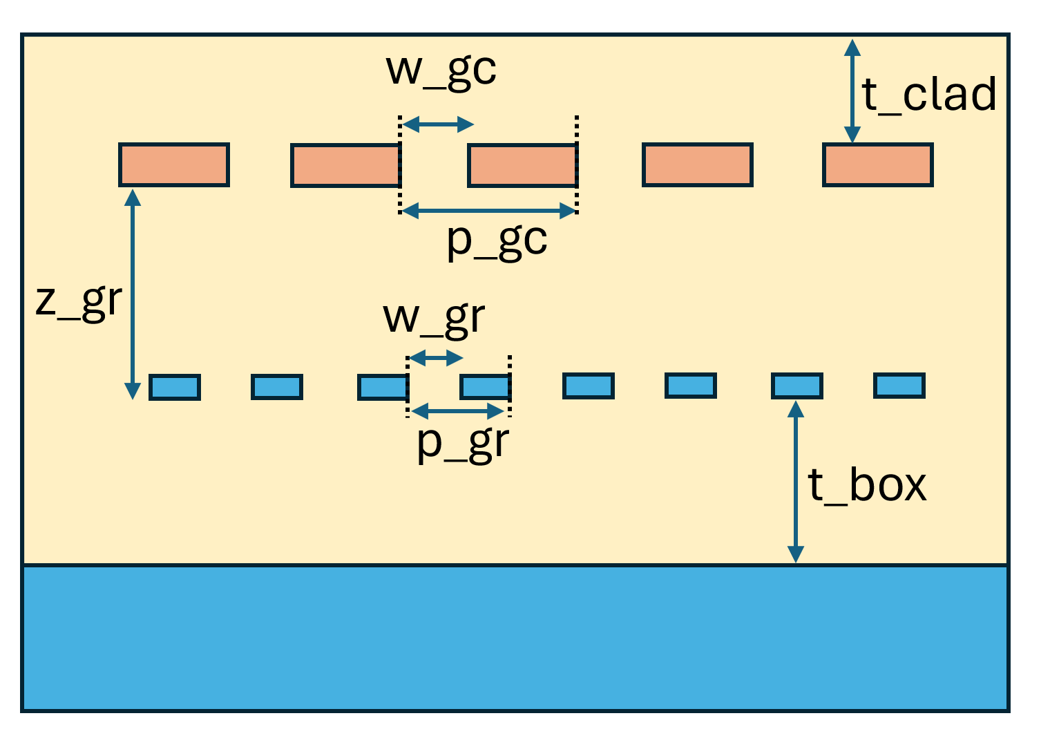
def make_2D_SiN_grating(w_gc: float, p_gc: float) -> td.Structure:
    """
    Creates a 2D SiN grating structure.

    Parameters:
        w_gc (float): Width of the etched region.
        p_gc (float): Period of the grating.

    Returns:
        td.Structure: The resulting grating structure.
    """
    gratings = 0
    # Iterate to create each period of the grating
    for i in range(n_gc):
        # Add a box for each grating period
        gratings += td.Box.from_bounds(
            rmin=(w_gc + i * p_gc, -inf_eff, 0), rmax=((i + 1) * p_gc, inf_eff, t_SiN)
        )

    return td.Structure(geometry=gratings, medium=SiN)


waveguide = td.Structure(
    geometry=td.Box.from_bounds(rmin=(-inf_eff, -inf_eff, 0), rmax=(0, inf_eff, t_SiN)),
    medium=SiN,
)

oxide_layer = td.Structure(
    geometry=td.Box.from_bounds(
        rmin=(-inf_eff, -inf_eff, -inf_eff), rmax=(inf_eff, inf_eff, t_SiN + t_clad)
    ),
    medium=SiO2,
)


def make_2D_SiN_grating_sim(w_gc: float, p_gc: float, x_fiber: float) -> td.Simulation:
    """
    Creates a simulation for a 2D SiN grating coupler.

    Parameters:
        w_gc (float): Width of the etched region.
        p_gc (float): Period of the grating.
        x_fiber (float): x-position of the fiber center.

    Returns:
        td.Simulation: The Tidy3D simulation object.
    """
    gratings = make_2D_SiN_grating(w_gc, p_gc)  # Create the grating structure

    # Create a Gaussian beam source representing the input fiber mode
    gaussian_beam = td.GaussianBeam(
        center=(x_fiber, 0, t_SiN + t_clad + lda0 / 4),
        size=(2 * mfd, td.inf, 0),
        source_time=td.GaussianPulse(freq0=freq0, fwidth=fwidth),
        pol_angle=np.pi / 2,
        angle_theta=theta,
        angle_phi=0,
        direction="-",
        waist_radius=mfd / 2,
        waist_distance=0,
    )

    # Simulation domain box
    sim_box = td.Box.from_bounds(
        rmin=(-lda0, 0, -lda0), rmax=(n_gc * p_gc + lda0, 0, t_SiN + t_clad + lda0)
    )

    # Create the simulation
    sim = td.Simulation(
        center=sim_box.center,
        size=sim_box.size,
        grid_spec=grid_spec,
        run_time=run_time,
        structures=[oxide_layer, gratings, waveguide],
        sources=[gaussian_beam],
        monitors=[mode_monitor],
        boundary_spec=boundary_spec,
    )
    return sim

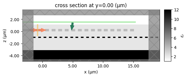
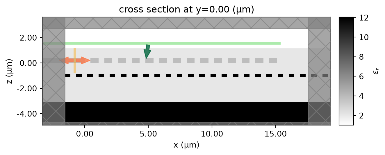
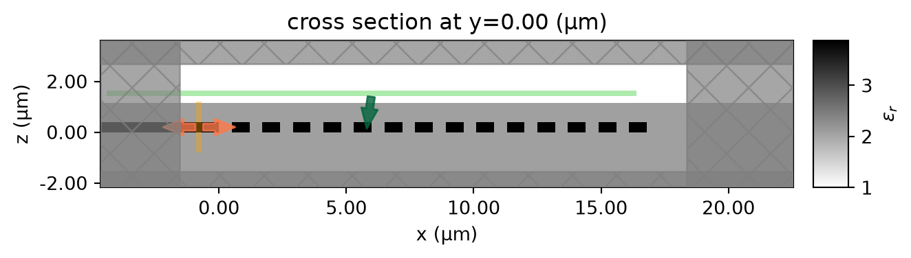
Create a single simulation to verify the setup and visualize the permittivity distribution.

sim = make_2D_SiN_grating_sim(w_gc=0.5, p_gc=1.2, x_fiber=6)
sim.plot_eps(y=0)
plt.show()

def coupling_efficiency(sim_data: td.SimulationData) -> dict:
    """
    Calculates the coupling efficiency from simulation data.

    Parameters
    ----------
    sim_data : td.SimulationData
        The simulation data containing mode amplitudes.

    Returns
    -------
    dict
        A dictionary containing the coupling efficiency in dB.
    """
    # Extract the amplitude of the fundamental mode (mode_index=0) propagating in the backward direction ("-") at the central frequency (freq0)
    amp = sim_data["mode"].amps.sel(mode_index=0, direction="-", f=freq0).values
    return {"coupling efficiency": 20 * np.log10(np.abs(amp))}

Now we are ready to perform the parameter sweep (grid search) using Tidy3D’s Design plugin.

# Define parameters and bounds
params = [
    tdd.ParameterFloat(name="w_gc", span=(0.4, 0.5), num_points=6),
    tdd.ParameterFloat(name="p_gc", span=(1.0, 1.2), num_points=6),
    tdd.ParameterFloat(name="x_fiber", span=(4.8, 5.2), num_points=5),
]

# Design optimization method (grid search)
method = tdd.MethodGrid()

# Create a design space and run the sweep
design_space = tdd.DesignSpace(method=method, parameters=params, path_dir="./data")
results = design_space.run(make_2D_SiN_grating_sim, coupling_efficiency)

14:01:13 UTC Running 180 Simulations

After the sweep is done, we can pick the optimal design parameters.

df = results.to_dataframe()  # Convert the results to a pandas DataFrame

# Pick the best design
best_row = df.loc[df["coupling efficiency"].idxmax()]
best_w_gc, best_p_gc, best_x_fiber = best_row[["w_gc", "p_gc", "x_fiber"]]
df.sort_values(by="coupling efficiency", ascending=False)

180 rows × 4 columns

Periodic Si Grating Reflector Design

To improve the coupling efficiency of the grating coupler, we add a bottom grating in the silicon layer to reflect leakage light upwards. We need to optimize the grating period and duty cycle to achieve maximum reflection.

def make_2D_Si_grating(w_gr: float, p_gr: float, z_gr: float) -> "td.Structure":
    """
    Creates a 2D silicon grating structure.

    Args:
        w_gr: Width of the etched region.
        p_gr: Period of the grating.
        z_gr: The z-coordinate of the bottom surface of the grating.

    Returns:
        A Tidy3D Structure object representing the entire grating.
    """
    offset = -2  # Initial offset for the grating placement

    # Loop to create multiple grating teeth
    gratings = 0
    for i in range(50):
        gratings += td.Box.from_bounds(
            rmin=(offset + w_gr + i * p_gr, -inf_eff, -z_gr),
            rmax=(offset + (i + 1) * p_gr, inf_eff, -z_gr + t_Si),
        )

    return td.Structure(geometry=gratings, medium=Si)


# Create a Gaussian beam at the optimal position
gaussian_beam = td.GaussianBeam(
    center=(best_x_fiber, 0, t_SiN + t_clad + lda0 / 4),
    size=(2 * mfd, td.inf, 0),
    source_time=td.GaussianPulse(freq0=freq0, fwidth=fwidth),
    pol_angle=np.pi / 2,
    angle_theta=theta,
    angle_phi=0,
    direction="-",
    waist_radius=mfd / 2,
    waist_distance=0,
)


def make_2D_Si_grating_sim(w_gr: float, p_gr: float, z_gr: float = 1) -> "td.Simulation":
    """
    Creates a Tidy3D simulation for a 2D silicon grating.

    Args:
        w_gr: Width of the etched region.
        p_gr: Period of the grating.
        z_gr: The z-coordinate of the bottom surface of the grating.

    Returns:
        A Tidy3D Simulation object.
    """
    # Create the grating structure
    gratings = make_2D_Si_grating(w_gr, p_gr, z_gr)

    # Define the substrate structure
    substrate = td.Structure(
        geometry=td.Box.from_bounds(
            rmin=(-inf_eff, -inf_eff, -inf_eff), rmax=(inf_eff, inf_eff, -z_gr - t_box)
        ),
        medium=Si,
    )

    # Define a flux monitor to measure reflection
    flux_monitor = td.FluxMonitor(
        center=(0, 0, t_SiN + t_clad + lda0 / 2),
        size=(td.inf, td.inf, 0),
        freqs=[freq0],
        normal_dir="+",
        name="flux",
    )

    # Simulation domain box
    sim_box = td.Box.from_bounds(
        rmin=(-lda0, 0, -z_gr - t_box - lda0),
        rmax=(20 * p_gr + lda0, 0, t_SiN + t_clad + lda0),
    )

    # Create the simulation
    sim = td.Simulation(
        center=sim_box.center,
        size=sim_box.size,
        grid_spec=grid_spec,
        run_time=run_time,
        structures=[oxide_layer, gratings, substrate],
        sources=[gaussian_beam],
        monitors=[flux_monitor],
        boundary_spec=boundary_spec,
    )
    return sim

Visualize the simulation setup.

sim = make_2D_Si_grating_sim(w_gr=0.2, p_gr=0.5)
sim.plot(y=0)
plt.show()

def reflectivity(sim_data: td.SimulationData) -> dict:
    """
    Extracts the reflectivity from the simulation data.

    Parameters:
        sim_data (td.SimulationData): The simulation data containing flux results.

    Returns:
        dict: A dictionary containing the reflectivity values.
    """
    # Extract the flux values from the simulation data
    r = sim_data["flux"].flux.values
    return {"reflectivity": r}

Similar to the previous section, we will perform a parameter sweep to optimize the Si grating period and duty cycle.

# Design parameters and bounds
params = [
    tdd.ParameterFloat(name="w_gr", span=(0.3, 0.5), num_points=11),
    tdd.ParameterFloat(name="p_gr", span=(0.7, 1.0), num_points=11),
]

# Perform parameter sweep
design_space = tdd.DesignSpace(method=method, parameters=params, path_dir="./data")
results = design_space.run(make_2D_Si_grating_sim, reflectivity)

14:04:28 UTC Running 121 Simulations

From the results, we find the parameters that yield the highest reflection.

df = results.to_dataframe()

best_row = df.loc[df["reflectivity"].idxmax()]
best_w_gr, best_p_gr = best_row[["w_gr", "p_gr"]]

df.sort_values(by="reflectivity", ascending=False)

121 rows × 3 columns

Interlayer Distance Optimization

Here we combine the optimized SiN grating and the optimized Si reflector into a single simulation and optimize the vertical separation z_gr to ensure constructive interference and therefore maximum coupling efficiency.

def make_2D_full_grating_sim(z_gr: float) -> td.Simulation:
    """
    Creates a simulation of the full coupler structure including SiN and Si gratings.

    Parameters
    ----------
    z_gr : float
        The z-position for the Si grating structure.

    Returns
    -------
    td.Simulation
        Tidy3D simulation object.
    """
    # Create the SiN grating structure using optimal width and period
    gratings_SiN = make_2D_SiN_grating(best_w_gc, best_p_gc)

    # Create the Si grating structure using optimal width, period, and the given z-position
    gratings_Si = make_2D_Si_grating(best_w_gr, best_p_gr, z_gr)

    # Define the silicon substrate structure
    substrate = td.Structure(
        geometry=td.Box.from_bounds(
            rmin=(-inf_eff, -inf_eff, -inf_eff), rmax=(inf_eff, inf_eff, -z_gr - t_box)
        ),
        medium=Si,
    )

    # Calculate the SiN grating length
    l = best_p_gc * n_gc

    # Simulation domain box
    sim_box = td.Box.from_bounds(
        rmin=(-lda0, 0, -z_gr - t_box - lda0), rmax=(l + lda0, 0, t_SiN + t_clad + lda0)
    )

    # Construct the simulation object
    sim = td.Simulation(
        center=sim_box.center,
        size=sim_box.size,
        grid_spec=grid_spec,
        run_time=run_time,
        structures=[oxide_layer, gratings_SiN, gratings_Si, waveguide, substrate],
        sources=[gaussian_beam],
        monitors=[mode_monitor],
        boundary_spec=boundary_spec,
    )
    return sim

Visualize and verify the simulation setup.

sim = make_2D_full_grating_sim(2)

sim.plot_eps(y=0)
plt.show()

Now we perform parameter sweep of the interlayer distance to maximize the coupling efficiency.

# Design parameter and bound
params = [
    tdd.ParameterFloat(name="z_gr", span=(1, 2), num_points=21),
]

# Perform parameter sweep
design_space = tdd.DesignSpace(method=method, parameters=params, path_dir="./data")
results = design_space.run(make_2D_full_grating_sim, coupling_efficiency)

# Plot the coupling efficiency as a function of z_gr
df = results.to_dataframe()
plt.plot(df["z_gr"], df["coupling efficiency"], marker="o")
plt.xlabel("z_gr")
plt.ylabel("Coupling efficiency (dB)")
plt.grid(True)
plt.show()

# Extract the best z_gr
best_row = df.loc[df["coupling efficiency"].idxmax()]
best_z_gr = best_row["z_gr"]
df.sort_values(by="coupling efficiency", ascending=False)

14:06:38 UTC Running 21 Simulations