Two-Segment Silicon Microring Modulator

Download notebook (.zip)

---

Learning objectives

By the end of this tutorial, you will know how to:

• Build an analytical waveguide model for passive and active (phase-shifting) segments, parameterized by effective index, group index, loss, and $V_\pi L$.
• Replace a full-wave S-matrix with a compact model: characterize a directional coupler with a coarse full-wave simulation, then substitute it with an analytical DirectionalCouplerModel that preserves power coupling for efficient, fine-grained frequency sweeps.
• Run time-domain electro-optic simulations by driving the modulator with PRBS electrical waveforms and observing the recovered optical and electrical signals.
• Generate an eye diagram from the detector output to evaluate signal integrity at the target symbol rate.

---

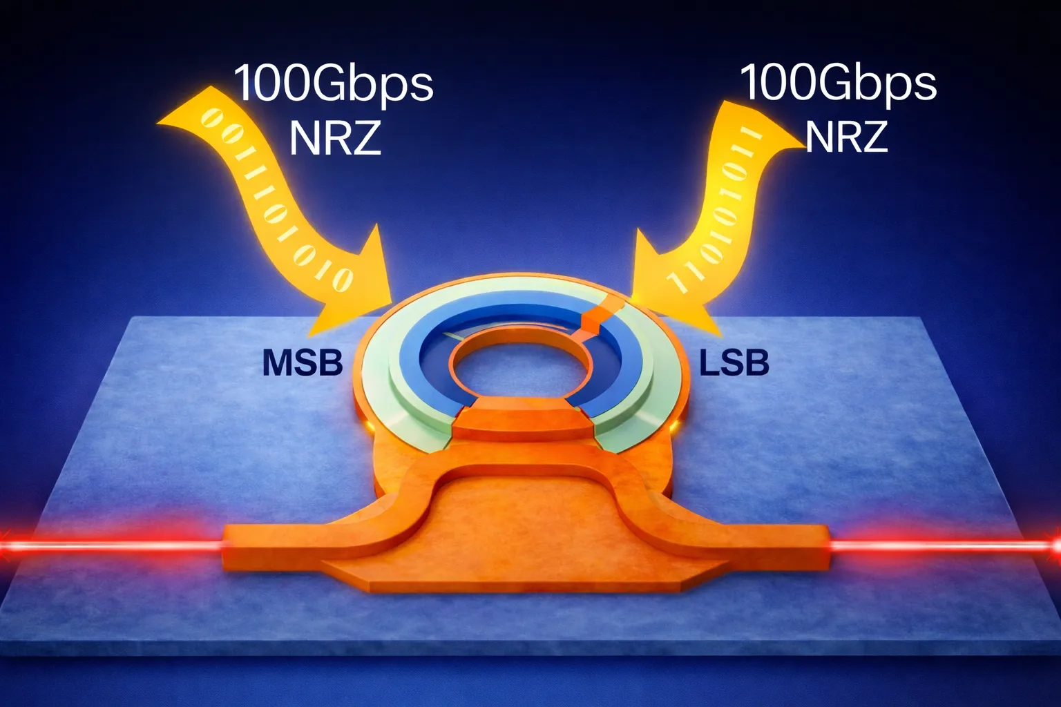
In this notebook, we develop a compact, physics-informed simulation replica of the two-segment silicon microring modulator reported in [1]. Rather than relying on full-wave electromagnetic simulations throughout, we combine analytical device models, circuit-level abstractions, and time-domain signal modeling to reproduce the key behaviors observed experimentally, while maintaining computational efficiency and transparency.

The workflow begins by defining the waveguide geometry and extracting the effective and group indices using a mode solver. A directional coupler is first characterized using a coarse full-wave S-matrix calculation, after which it is replaced by an analytical coupler model that preserves power coupling while discarding phase details. Because, certain physical effects—such as charge-dependent propagation loss and electro-optic modulation behavior—cannot be conveniently incorporated at this stage.

We then construct a two-segment microring modulator composed of an MSB and an LSB depletion-mode phase shifter, along with a passive waveguide section that completes the ring. Each active segment is modeled using an analytic waveguide with explicit control over $V_\pi L$, propagation loss, voltage-dependent loss, and RC-limited bandwidth via a first-order time constant. This structure naturally supports independent electrical driving of the MSB and LSB segments, mirroring the optical-DAC concept introduced in the reference work.

After validating the static behavior through frequency-domain S-matrix analysis—capturing resonance positions, extinction, and voltage-dependent wavelength shifts—we move to time-domain simulation. A CW laser is detuned from resonance to operate at the point of maximum slope, electrical PRBS-driven trapezoid waveforms are applied to the modulator ports, and a bandwidth-limited photodiode model converts the optical output into an electrical signal.

Finally, we evaluate large-signal performance by plotting eye diagrams from the detector output, demonstrating how the compact model captures the essential dynamics of high-speed microring modulation. Overall, this notebook serves as a clear, extensible reference implementation for resonant modulator modeling, bridging device physics, circuit abstraction, and system-level signal integrity within a single, efficient simulation framework.

References

1. Yuan, Yuan, et al. “A 5× 200 Gbps microring modulator silicon chip empowered by two-segment Z-shape junctions.” Nature Communications, 2024 15 (1), 918, doi: 10.1038/s41467-024-45301-3

import numpy as np
import photonforge as pf
import photonforge.abstract as pfa
from matplotlib import pyplot as plt

import tidy3d as td

td.config.logging.level = "ERROR"

Simulation Parameters

In this section, we define the nominal silicon photonic waveguide and microring geometry (all lengths in µm), along with the baseline electro-optic and RF parameters used throughout the notebook.

We parameterize the waveguide cross-section using the core width/height and slab height, then define a nominal microring radius and the coupling-section geometry (coupling length and bus-to-ring gap). Since the coupling region is treated as a straight interaction section, we adjust the effective bend radius so that the combined curved + straight segments match the intended nominal circumference.

We then split the ring’s phase-shifting region into two depletion-mode segments:

• an LSB segment (shorter),
• an MSB segment (longer),

and assign the remaining circumference to an additional passive waveguide segment. Finally, we specify optical loss and modulation figures of merit (e.g., $\alpha$ in dB/cm and $V_\pi L$ in V.cm) and the extracted RC-limited bandwidth targets for each segment.

# Geometry details (all units in um)
w_core = 0.5
h_core = 0.22
h_slab = 0.09

# Microring and coupler geometry
nominal_radius = 12
coupling_length = 4
radius = nominal_radius - coupling_length / np.pi
gap = 0.18

# Two-segment modulator lengths (LSB/MSB) and remaining passive length
lsb_length = 20
msb_length = 40
extra_wg_length = 2 * np.pi * nominal_radius - lsb_length - msb_length

# Optical loss model and voltage-dependent loss term (in dB/cm and dB/cm/V)
alpha_db_cm = 133
dloss_dv_db_cm_v = -3

# Modulation efficiency (V*pi*L in V*cm)
msb_vpiL_v_cm = 0.69
lsb_vpiL_v_cm = 0.53

# RC-limited bandwidth targets for each segment (Hz)
f_rc_msb = 64.0e9
f_rc_lsb = 79.1e9

# The optical carrier wavelength (in um) and the corresponding carrier frequency
lambda0 = 1.31
freq0 = td.C_0 / lambda0

# Coarse frequency grid spanning a narrow O-band window around the carrier.
# This grid is used to run the coarse full-wave sweep of the directional coupler.
freqs_coarse = pf.C_0 / np.linspace(lambda0 - 0.05, lambda0 + 0.05, 11)

# Define a fine wavelength sweep to resolve the microring resonance
lda_fine = np.linspace(1.306, 1.312, 1001)
freqs_fine = pf.C_0 / lda_fine

Next, we construct a basic silicon photonics technology object using the previously defined core and slab thicknesses and register it as the default technology. We then define a virtual electrical port (virtual_port_spec) that will be used for both electrical excitation of the modulators and electrical signal readout from the detector and the source.

tech = pf.basic_technology(core_thickness=h_core, slab_thickness=h_slab, rib_width=0.5)
pf.config.default_technology = tech
elec_vir = pf.virtual_port_spec(classification="electrical")
opt_vir = pf.virtual_port_spec(classification="optical")

Rib Waveguide Mode Analysis

In this section, we solve for the fundamental optical mode of the rib waveguide (which will be used in the microring modulator) and extract its frequency-dependent effective index $n_\mathrm{eff}(f)$ and group index $n_g(f)$.

We run the built-in mode solver on the coarse frequency grid freqs_coarse (a narrow band around the carrier wavelength), visualize the electric field profile of the fundamental mode for sanity checking, and wrap the resulting $n_\mathrm{eff}$ and $n_g$ samples in pf.Interpolator objects.

The AnalyticWaveguideModel and PhaseModTimeStepper used in the rest of the notebook both accept Interpolator inputs for $n_\mathrm{eff}$ and $n_g$, so chromatic dispersion is incorporated directly into the compact model: any S-matrix sweep or time-domain run automatically evaluates the indices at the relevant frequency, with no need for a separate dispersion-correction step.

# Solve the rib-waveguide modes across the coarse frequency grid
mode_solver = pf.port_modes("Rib", freqs_fine, group_index=True)

# Plot the electric field profile of the solved fundamental mode at the carrier frequency
mode_solver.plot_field("E", f=freqs_fine[len(freqs_fine) // 2])

# Extract the frequency-dependent group and effective indices of the fundamental mode
n_group_vs_f = mode_solver.data.n_group.isel(mode_index=0).values
n_eff_vs_f = mode_solver.data.n_eff.isel(mode_index=0).values

# Wrap the samples in pf.Interpolator objects so that the analytic waveguide
# model and the phase-modulator time stepper natively see n_eff(f) and n_g(f).
n_eff = pf.Interpolator(freqs_fine, n_eff_vs_f)
n_group = pf.Interpolator(freqs_fine, n_group_vs_f)

Uploading task 'Mode-ModeSolver…'
Starting task 'Mode-ModeSolver': https://tidy3d.simulation.cloud/workbench?taskId=mo-5044f2b6-84ae-4519-9aca-01e35692459c
Downloading data from 'Mode-ModeSolver'…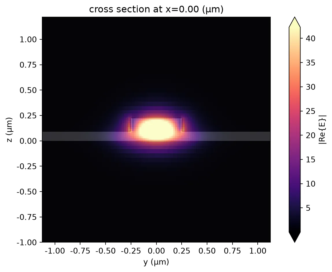

Directional Coupler for Ring–Bus Interaction

In this section, we construct the directional coupler that mediates optical power exchange between the straight bus waveguide and the microring.

dc = pf.parametric.s_bend_ring_coupler(
    port_spec="Rib",
    coupling_distance=gap + w_core,
    coupling_length=coupling_length,
    radius=radius,
    s_bend_length=10,
    s_bend_offset=2,
    model=pf.Tidy3DModel(grid_spec=12)
)
dc

After performing a full-wave S-matrix calculation of the directional coupler, we switch to an analytical DirectionalCouplerModel for subsequent simulations.

Why use a compact coupler model? Trade-offs and motivation

What we gain:

• Speed: Full-wave S-matrix calculations are expensive. Replacing them with a compact model lets us evaluate the circuit on a fine frequency grid (e.g., many points over a narrow wavelength range), which is essential to resolve resonances, extinction, and tuning curves accurately. Doing the same sweep with full-wave Tidy3D would require a large number of simulations and become prohibitively slow.
• Controlled physics: In an analytical coupler we discard detailed phase and spatial information from the full-wave solution. That allows us to add propagation loss (e.g., doping-dependent loss) and electro-optic modulation ($V_\pi L$, voltage-dependent loss, RC bandwidth) in a transparent, explicit way later in the waveguide and modulator models. Those effects are difficult or inconvenient to incorporate directly into a single full-wave coupler run.
• Reuse: One coarse full-wave run gives us coupling ($\kappa$) and through ($t$) coefficients; the same compact coupler is then reused everywhere in the netlist.

What we give up:

• Spatial and phase detail: The full-wave solution contains exact phase and field distributions. The analytical coupler preserves power coupling (magnitude) but not the full phase response; for resonant circuits we often care more about power coupling and round-trip phase, which we capture via the ring waveguide model.
• Wavelength dependence: We take $\kappa$ and $t$ at a single (center) frequency. Over a narrow band around the carrier this is usually sufficient; for very wide bands you might need to re-extract or use a frequency-dependent compact model.

Here, we extract $\kappa$ and $t$ from the center frequency of a coarse sweep and build a lossless analytical coupler that can be reused efficiently across the notebook.

# Compute the full-wave S-matrix of the directional coupler on the coarse grid
s_matrix = dc.s_matrix(freqs_coarse, model_kwargs={"inputs": ["P0"]})

# Plot the S-matrix magnitude responses
fig, ax = pf.plot_s_matrix(s_matrix)

# Extract coupling and through coefficients at the center frequency
kappa = np.abs(s_matrix[("P0@0", "P3@0")][len(freqs_coarse) // 2])
trans = np.abs(s_matrix[("P0@0", "P2@0")][len(freqs_coarse) // 2])

# Build an analytical directional coupler model using extracted coefficients
analytical_dc = pf.DirectionalCouplerModel(t=trans, c=-1j * kappa).black_box_component(
    opt_vir
)

Uploading task 'P0@0…'
Starting task 'P0@0': https://tidy3d.simulation.cloud/workbench?taskId=fdve-97067580-4389-4c3e-b4ac-3219e3082878
Downloading data from 'P0@0'…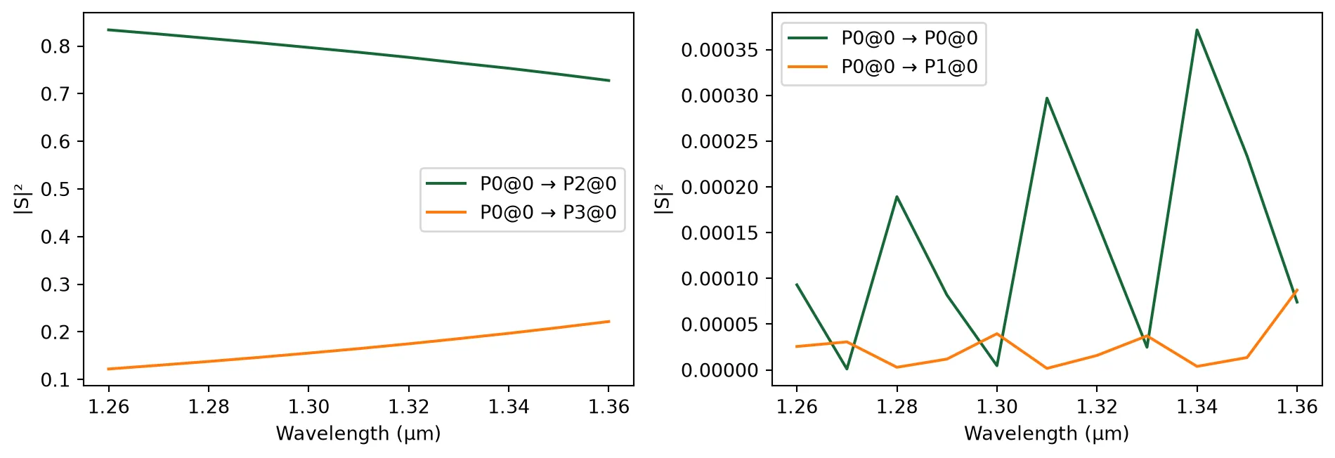

Microring Modulator Assembly

Now, we define a parametric waveguide component that serves as the reusable building block for constructing the microring modulator.

We use the same function to represent both:

• passive ring sections (no electrical port, no time-domain modulation), and
• active modulator sections (with a virtual electrical port and an attached phase-modulation time stepper).

The component is built from the AnalyticWaveguideModel parameterized by $n_\mathrm{eff}$, $n_g$, and a reference frequency. For active sections, we include modulation physics through $V_\pi L$, propagation loss, voltage-dependent loss, and a first-order RC response with a $-3~\mathrm{dB}$ cutoff frequency $f_\mathrm{3dB} = f_\mathrm{RC}$, via the PhaseModTimeStepper for time-domain simulations.

# Create a reusable parametric waveguide component for passive and active ring sections
@pf.parametric_component
def create_wg(
    n_eff=n_eff,
    length=2 * np.pi * radius,
    n_group=n_group,
    reference_frequency=freq0,
    v_piL=1e10,
    propagation_loss=alpha_db_cm * 1e-4,
    dloss_dv=dloss_dv_db_cm_v * 1e-4,
    f_rc=1e12,
    is_modulator=True,
    name="Analytic Waveguide",
):
    model = pf.AnalyticWaveguideModel(
        n_eff=n_eff,
        length=length,
        n_group=n_group,
        reference_frequency=reference_frequency,
        v_piL=v_piL,
        propagation_loss=propagation_loss,
        dloss_dv=dloss_dv,
    )
    wg = model.black_box_component(port_spec=opt_vir, name=name)
    if is_modulator:
        wg.add_port(pf.Port(0j, 0, elec_vir))
        model.time_stepper = pf.PhaseModTimeStepper(
            n_eff=n_eff,
            length=length,
            n_group=n_group,
            v_piL=v_piL,
            propagation_loss=propagation_loss,
            dloss_dv=dloss_dv,
            f_3dB=f_rc,
        )

    return wg

create_wg()

Next, we construct the full microring resonator modulator (MRM) by combining:

• the analytical directional coupler (bus-to-ring coupling),
• an MSB active phase-shifter segment,
• an LSB active phase-shifter segment, and
• an extra passive waveguide segment that completes the ring circumference.

We parameterize the active segments independently to allow different $n_\mathrm{eff}$, lengths, $V_\pi L$, and RC-limited bandwidths ($f_\mathrm{RC}$). The MSB and LSB sections each expose a virtual electrical port for driving the modulator segments, while the passive section has no electrical interface.

We then define a netlist describing the instances, their virtual optical interconnections around the ring, the external ports (two optical ports on the coupler and two electrical ports for MSB/LSB), and attach a circuit-level model to enable compact system simulation of the full resonant device.

# Build a two-segment microring modulator (MRM) using an analytical coupler and analytic waveguide sections
@pf.parametric_component
def create_mrm(
    msb_n_eff=n_eff,
    lsb_n_eff=n_eff,
    extra_wg_n_eff=n_eff,
    n_group=n_group,
    msb_length=msb_length,
    lsb_length=lsb_length,
    extra_wg_length=extra_wg_length,
    msb_vpiL=msb_vpiL_v_cm * 1e4,
    lsb_vpiL=lsb_vpiL_v_cm * 1e4,
    f_rc_msb=f_rc_msb,
    f_rc_lsb=f_rc_lsb,
    reference_frequency=freq0,
):

    msb_wg = create_wg(
        n_eff=msb_n_eff,
        n_group=n_group,
        length=msb_length,
        reference_frequency=reference_frequency,
        v_piL=msb_vpiL,
        f_rc=f_rc_msb,
        name="MSB",
    )
    lsb_wg = create_wg(
        n_eff=lsb_n_eff,
        n_group=n_group,
        length=lsb_length,
        reference_frequency=reference_frequency,
        v_piL=lsb_vpiL,
        f_rc=f_rc_lsb,
        name="LSB",
    )
    extra_wg = create_wg(
        n_eff=extra_wg_n_eff,
        n_group=n_group,
        length=extra_wg_length,
        reference_frequency=reference_frequency,
        is_modulator=False,
    )
    # Define the netlist for a microring resonator
    netlist_mrm = {
        "name": "Microring Modulator",  # name of the component
        "instances": {
            "dc": analytical_dc,
            "msb": {"component": msb_wg, "origin": (0, 5), "rotation": 90},
            "lsb": {"component": lsb_wg, "origin": (20, 45), "rotation": -90},
            "extra": {"component": extra_wg, "origin": (20, 5), "rotation": 90},
        },
        "virtual connections": [
            (("msb", "P0"), ("dc", "P1")),
            (("msb", "P1"), ("lsb", "P0")),
            (("lsb", "P1"), ("extra", "P1")),
            (("extra", "P0"), ("dc", "P3")),
        ],
        # Define external ports
        "ports": [("dc", "P0"), ("dc", "P2"), ("msb", "E0"), ("lsb", "E0")],
        # Assign a CircuitModel to simulate the entire microring
        "models": [(pf.CircuitModel(), "Circuit")],
    }

    # Build the microring resonator from the netlist
    mrm = pf.component_from_netlist(netlist_mrm)

    return mrm

create_mrm()

LayoutSchematic

Then, we instantiate the microring modulator and compute its optical S-matrix over a fine wavelength sweep around the O-band carrier. Using a dense wavelength grid is essential for resonant devices because the resonance features are narrow and require high spectral resolution.

By plotting the through response, we observe a clear resonance dip at approximately 1309 nm, confirming that the ring resonance is captured by the circuit-level model of the assembled MRM.

# Instantiate the microring modulator
mrm = create_mrm()

# Compute the S-matrix of the microring over the fine frequency grid
s_matrix_mrm = mrm.s_matrix(freqs_fine)

# Plot the through-port transmission response to visualize the resonance dip
fig, ax = pf.plot_s_matrix(
    s_matrix_mrm, y="dB", input_ports=["P0"], output_ports=["P1"]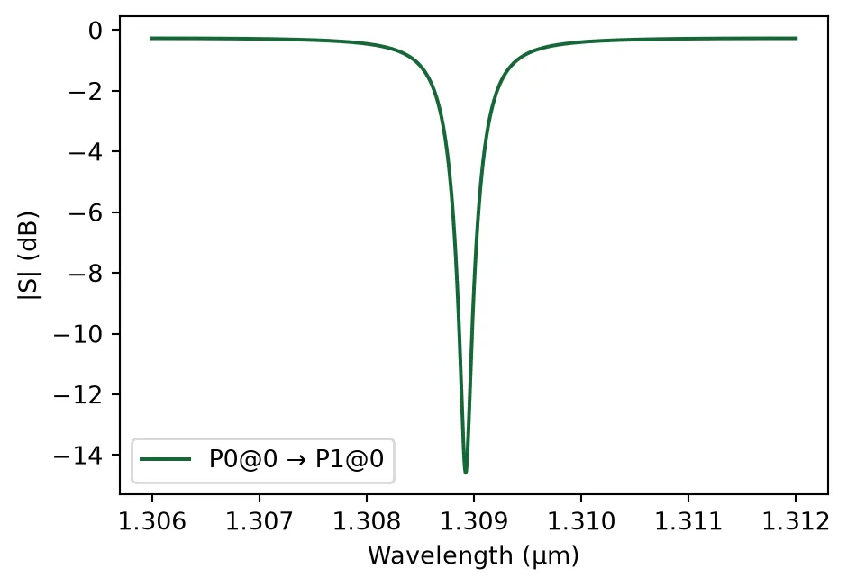
)

Voltage-Dependent Resonance Tuning

In this section, we analyze how the microring transmission spectrum shifts with applied junction voltage for the MSB and LSB modulator segments.

Although the physical device operates under reverse bias (negative voltage), we apply positive voltage values in the model for simplicity while keeping $V_\pi L$ positive. If we were to use negative voltages directly, we would need to assign negative values for $V_\pi L$ to preserve the correct modulation polarity. To avoid confusion, the plot legend explicitly displays the voltage with a negative sign to emphasize that these correspond to reverse-bias conditions.

For each voltage value, we:

• apply the voltage to only one segment at a time (MSB-only or LSB-only),
• compute the updated S-matrix over a fine wavelength grid,
• convert the through response to $|S|^2$ in dB, and
• extract the resonance wavelength as the wavelength at which the transmission is minimum.

# Reverse bias voltages
voltages = np.array([-0.5, 0, 1, 2, 3, 4])

# Initialize the figure
fig, ax = plt.subplots(1, 2, figsize=(10, 4))

res_wv_msb = np.zeros_like(voltages)
res_wv_lsb = np.zeros_like(voltages)
for i, v in enumerate(voltages):
    # Update only the MSB segment voltage while keeping LSB at 0 V
    updates_msb = {
        ("MSB", 0): {"model_updates": {"voltage": v}},
        ("LSB", 0): {"model_updates": {"voltage": 0}},
    }
    # Update only the LSB segment voltage while keeping MSB at 0 V
    updates_lsb = {
        ("MSB", 0): {"model_updates": {"voltage": 0}},
        ("LSB", 0): {"model_updates": {"voltage": v}},
    }
    # Compute the S-matrix under MSB-only and LSB-only bias conditions
    s_matrix_msb = mrm.s_matrix(freqs_fine, model_kwargs={"updates": updates_msb})
    s_matrix_lsb = mrm.s_matrix(freqs_fine, model_kwargs={"updates": updates_lsb})

    # Compute the through response in dB
    s_21_msb = 10 * np.log10(np.abs(s_matrix_msb[("P0@0", "P1@0")]) ** 2)
    s_21_lsb = 10 * np.log10(np.abs(s_matrix_lsb[("P0@0", "P1@0")]) ** 2)

    # Extract the resonance wavelength as the transmission minimum
    res_wv_msb[i] = lda_fine[np.argmin(s_21_msb)]
    res_wv_lsb[i] = lda_fine[np.argmin(s_21_lsb)]

    # Label voltage with negative sign to emphasize reverse-bias convention
    label = f"$V = {-v:.1f} V$"
    ax[0].plot(lda_fine * 1000, s_21_msb, label=label)
    ax[1].plot(lda_fine * 1000, s_21_lsb, label=label)

# Final plot formatting
ax[0].set_xlabel("Wavelength (nm)")
ax[0].set_ylabel("Through-port transmission $|S_{21}|^2$ (dB)")
ax[0].legend()
ax[0].set_xlim(1308.6, 1309.3)
ax[0].set_title("MSB segment: resonance vs. bias voltage")
ax[0].grid(True, alpha=0.3)
ax[1].set_xlabel("Wavelength (nm)")
ax[1].set_ylabel("Through-port transmission $|S_{21}|^2$ (dB)")
ax[1].legend()
ax[1].set_xlim(1308.6, 1309.3)
ax[1].set_title("LSB segment: resonance vs. bias voltage")
ax[1].grid(True, alpha=0.3)
fig.suptitle("Microring transmission vs. wavelength at different bias voltages", y=1.02)
plt.tight_layout()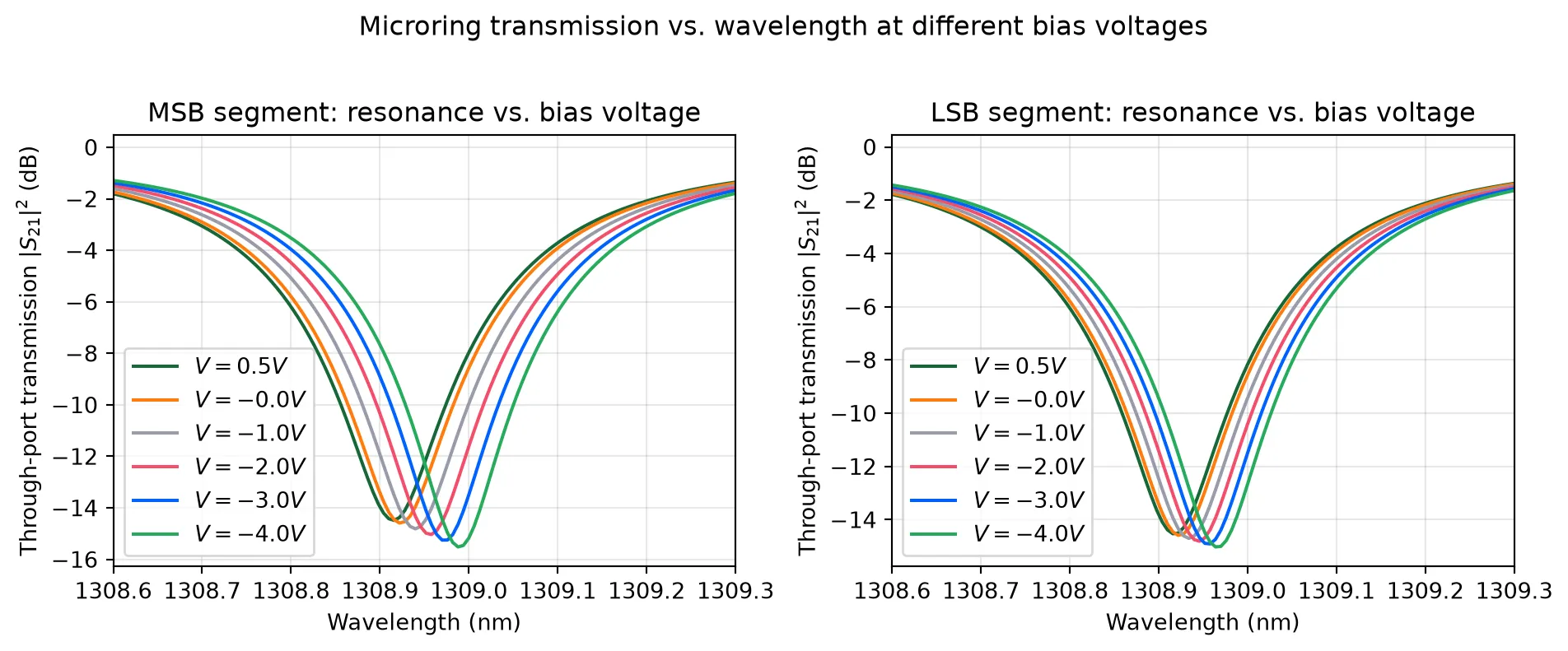

We also quantify the voltage-induced resonance shift for the MSB and LSB segments by plotting the extracted resonance wavelength as a function of bias voltage.

As before, the horizontal axis is shown using negative voltages to reflect the physical reverse-bias operation, while the model internally uses positive voltages. We then perform a linear fit to extract the tuning efficiency in units of pm/V for each segment, which can be directly compared against the reported experimental values.

# Plot resonance wavelength versus bias voltage for MSB and LSB
fig, ax = plt.subplots(1, 2, figsize=(10, 4))

# MSB resonance shift
ax[0].plot(-voltages, res_wv_msb * 1e6, "ro", label="Simulated resonance")
ax[0].set_ylabel("Resonance wavelength (pm)")
ax[0].set_xlabel("Bias voltage (V, reverse bias)")
ax[0].set_title("MSB: resonance shift vs. voltage")

# Linear fit for MSB
msb_fit_params = np.polyfit(voltages, res_wv_msb * 1e6, 1)
slope_msb = msb_fit_params[0]
intercept_msb = msb_fit_params[1]

# Fitted line: y = m*x + c
fit_msb = slope_msb * voltages + intercept_msb
ax[0].plot(-voltages, fit_msb, "b--", label=f"Fit ({slope_msb:.1f} pm/V)")
ax[0].legend()

# LSB resonance shift
ax[1].plot(-voltages, res_wv_lsb * 1e6, "ro", label="Simulated resonance")
ax[1].set_ylabel("Resonance wavelength (pm)")
ax[1].set_xlabel("Bias voltage (V, reverse bias)")
ax[1].set_title("LSB: resonance shift vs. voltage")

# Linear fit for LSB
lsb_fit_params = np.polyfit(voltages, res_wv_lsb * 1e6, 1)
slope_lsb = lsb_fit_params[0]
intercept_lsb = lsb_fit_params[1]

# Fitted line: y = m*x + c
fit_lsb = slope_lsb * voltages + intercept_lsb
ax[1].plot(-voltages, fit_lsb, "g--", label=f"Fit ({slope_lsb:.1f} pm/V)")
ax[1].legend()

plt.tight_layout()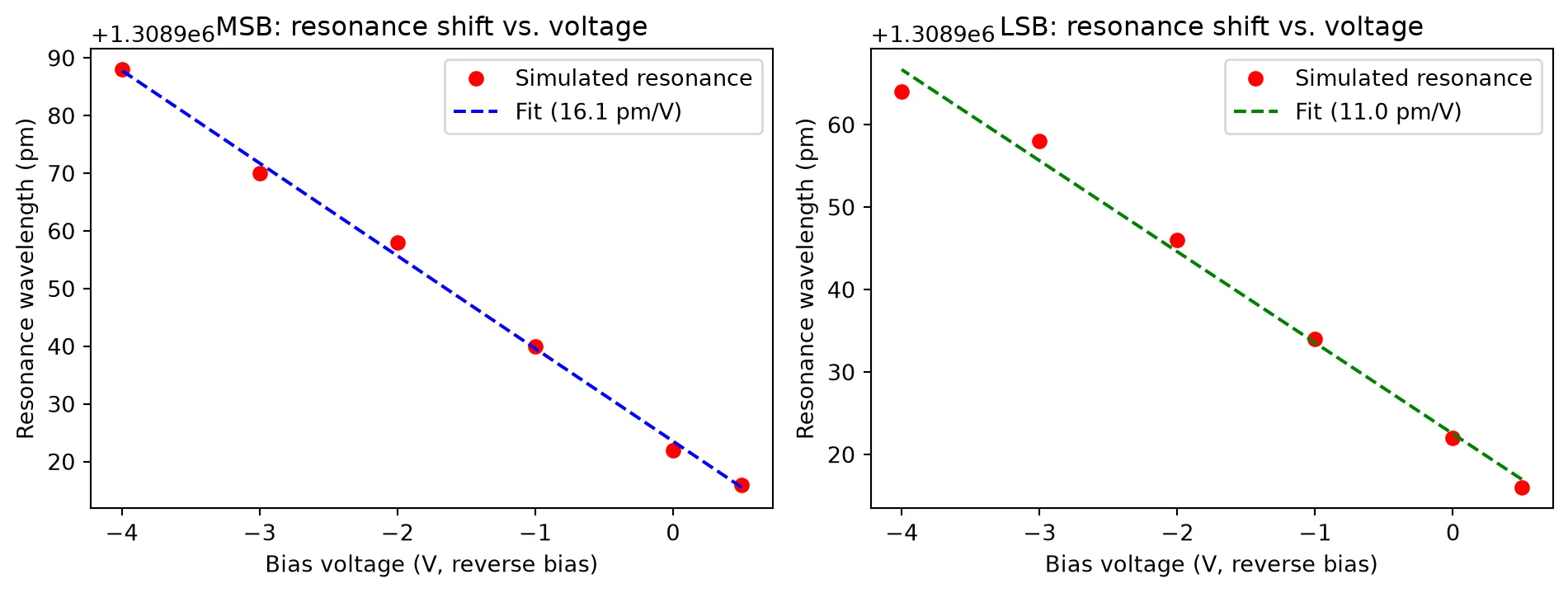

Full Time-Domain Dual-Segment MRM Testbench

In this section, we assemble a complete time-domain testbench for the two-segment microring modulator.

Electrical Drive Sources for Time-Domain Modulation

First, we define the time-domain electrical excitation used to drive the microring modulator segments.

PhotonForge operates on complex wave amplitudes, where electrical and optical signals are represented in terms of voltage-wave amplitudes rather than instantaneous power. As a result, the signal magnitude is proportional to the square root of power. To apply a desired physical voltage level to a port with characteristic impedance $Z_0$, the voltage values must therefore be scaled by $1/\sqrt{Z_0}$. In this example, we assume a default $50~\Omega$ impedance, which is why both the waveform amplitude and offset are divided by $\sqrt{50}$.

We set the symbol rate to $f_m = 100~\mathrm{GHz}$. For the MSB drive, the combination of offset + amplitude/2 defines the effective DC bias point applied to the junction. With the chosen parameters, this corresponds to a 3 V reverse-bias operating point, consistent with the device characterization. The LSB source is initially configured with zero amplitude and zero offset so that it can be enabled independently without modifying the circuit topology.

The code below implements these two voltage sources using pfa.signal_source.

f_m = 100e9
Z0 = 50.0

voltage_source_msb = pfa.signal_source(
    frequency=f_m,
    amplitude=1.6 / Z0**0.5,
    offset=2.2 / Z0**0.5,
    waveform="trapezoid",
    width=1,
    prbs=7,
    seed=123,
)

voltage_source_lsb = pfa.signal_source(
    frequency=f_m,
    amplitude=0,
    offset=0,
    waveform="trapezoid",
    width=1,
    prbs=7,
    seed=123,
)

Continuous-Wave Laser Source

Then, we define the optical input laser used for time-domain modulation simulations.

We intentionally detune the laser wavelength by 0.1 nm from the resonance to operate the microring close to the point of maximum transmission slope, where the modulation efficiency is highest. This operating point is commonly used in resonant modulators to maximize optical modulation amplitude for a given phase shift.

The laser is modeled as an ideal continuous-wave (CW) source with fixed optical power and frequency, implemented as a pfa.cw_laser. This abstraction provides a clean optical excitation without introducing additional modulation or noise sources.

lambda_laser = res_wv_msb[-2] - 0.0001  # detuned to operate close to maximum slope
f_laser = pf.C_0 / lambda_laser

laser = pfa.cw_laser(power=1e-3)

Photodiode Receiver

We also need to define a compact photodiode model to convert the modulated optical signal into an electrical waveform that we can monitor in the time domain.

We configure a pfa.photodiode using parameters consistent with a Keysight N1030A 65 GHz unamplified module, including responsivity, effective transimpedance gain from a 50 Ω load, saturation and dark current limits, thermal (Johnson) noise, and a finite receiver bandwidth modeled as a low-pass response with a specified roll-off.

The pfa.photodiode component already exposes an electrical output port (E0) alongside the optical input (P0), so it can be connected directly into the circuit netlist as an optical input / electrical output element.

# Setup for Keysight N1030A (65 GHz Unamplified Module)
detector = pfa.photodiode(
    responsivity=0.85,  # A/W (Typical for InGaAs)
    gain=50.0,  # V/A (Effective gain from 50 Ohm load)
    saturation_current=6.8e-3,  # A (Based on 8 mW max linear input)
    dark_current=10e-9,  # A (Typical 10 nA)
    thermal_noise=3.3e-22,  # A²/Hz (Johnson noise of 50 Ohm load)
    filter_frequency=65e9,  # Hz (65 GHz Bandwidth)
    roll_off=2,
    seed=123,  # Same noise in every run
)

Finally, we assemble the two-segment microring modulator by wiring together the optical and electrical building blocks into a single circuit netlist.

The netlist includes:

• the microring modulator (with separate MSB and LSB electrical ports),
• two independent electrical drive sources (MSB and LSB),
• a CW laser feeding the microring input, and
• a photodiode receiver that converts the modulated optical output into an electrical signal.

We connect each electrical source to its corresponding modulator segment (MSB-to-E0 and LSB-to-E1), route the laser into the microring input port, and route the microring through-port output into the detector. Finally, we expose only the detector’s electrical output as the external port of the composite component so that downstream simulations can directly probe the recovered electrical waveform.

The next cell defines the netlist as a dictionary (instances, virtual connections, exposed ports) and builds the composite component with component_from_netlist.

netlist_dual_segment = {
    "name": "Dual Segment MRM modulator",
    "instances": {
        "mrm": {"component": mrm, "origin": (10, 0)},
        "vs_msb": {"component": voltage_source_msb, "origin": (15, 5)},
        "vs_lsb": {"component": voltage_source_lsb, "origin": (30, 50)},
        "laser": {"component": laser, "rotation": 180},
        "detector": {"component": detector, "origin": (30, 0)},
    },
    "virtual connections": [
        (("vs_msb", "E0"), ("mrm", "E0")),  # Connect MSB source to MSB port
        (("vs_lsb", "E0"), ("mrm", "E1")),  # Connect LSB source to LSB port
        (("laser", "P0"), ("mrm", "P0")),
        (("detector", "P0"), ("mrm", "P1")),
    ],
    "ports": [("detector", "E0")],
    "models": [(pf.CircuitModel(), "Circuit")],
}

msb_modulator = pf.component_from_netlist(netlist_dual_segment)
msb_modulator

LayoutSchematic

Time-Domain Simulation of the Dual-Segment Microring Modulator

In this section, we run a time-domain simulation of the assembled dual-segment MRM testbench and observe the recovered electrical waveform at the detector output.

We define a discrete time grid with $N_\mathrm{steps}$ samples spaced by time_step. The circuit time stepper is set up with carrier_frequency=f_laser so that the rapidly rotating optical envelope at the laser frequency is handled internally by the simulator; this lets the time step be sized only by the RF modulation bandwidth rather than by the absolute optical frequency. Because $n_\mathrm{eff}$ and $n_g$ are already supplied as frequency-dependent Interpolator objects, the waveguide and phase-modulator models automatically evaluate them at the chosen carrier — no manual dispersion correction is required.

We also provide a frequency grid for the time stepper that spans a wide band around the carrier (here $\pm 200 f_m$) to capture modulation-induced sidebands. After resetting the time stepper state, we step the simulation forward, extract the detector electrical output, and use time-stepper monitors to directly read the source-port electrical wave amplitudes. We then plot both the input drive signals and the recovered electrical waveform over a short time window for inspection.

# Time-domain simulation parameters and time vector
time_step = 0.01 / f_m
N_steps = 100000
t = time_step * np.arange(N_steps)

# Resolve subcomponent references for monitor placement
refs = msb_modulator.references
vs_msb_ref = refs[1]
vs_lsb_ref = refs[2]

# Configure time-stepper with monitors on electrical source ports
ts = msb_modulator.setup_time_stepper(
    time_step=time_step,
    carrier_frequency=f_laser,
    time_stepper_kwargs={
        "frequencies": np.linspace(freq0 - 200 * f_m, freq0 + 200 * f_m, 100),
        "monitors": {
            "msb_src": vs_msb_ref["E0"],
            "lsb_src": vs_lsb_ref["E0"],
        },
    },
)

# Reset internal states before stepping
ts.reset()

# Run the time-domain simulation
outputs = ts.step(steps=N_steps, time_step=time_step)

# Extract detector electrical output waveform
output_signal = outputs["E0@0"]
msb_src_wave = outputs["msb_src@0+"]
lsb_src_wave = outputs["lsb_src@0+"]

# Convert monitored wave amplitudes to equivalent voltage at 50 Ohm for readability
v_msb_phys = np.real(msb_src_wave) * np.sqrt(Z0)
v_lsb_phys = np.real(lsb_src_wave) * np.sqrt(Z0)

# Plot input drive and detector output over a short time window
win = slice(1000, 4000)
fig, (ax1, ax2) = plt.subplots(2, 1, figsize=(10, 5), sharex=True)
ax1.plot(t[win] * 1e9, v_msb_phys[win], label=f"MSB source", color="C0")
ax1.plot(t[win] * 1e9, v_lsb_phys[win], label=f"LSB source", color="C1")
ax1.set_ylabel("Input voltage (V)")
ax1.set_title("Electrical drive signals from time-stepper monitors")
ax1.legend(loc="upper right")
ax1.grid(True, alpha=0.3)

ax2.plot(t[win] * 1e9, np.real(output_signal[win]), label="Detector output (real)")
ax2.set_xlabel("Time (ns)")
ax2.set_ylabel("Amplitude")
ax2.set_title("Recovered electrical waveform at detector output")
ax2.legend(loc="upper right")
ax2.grid(True, alpha=0.3)

fig.suptitle("Time-domain simulation: monitored input drive and output signal", y=1.02)
plt.tight_layout()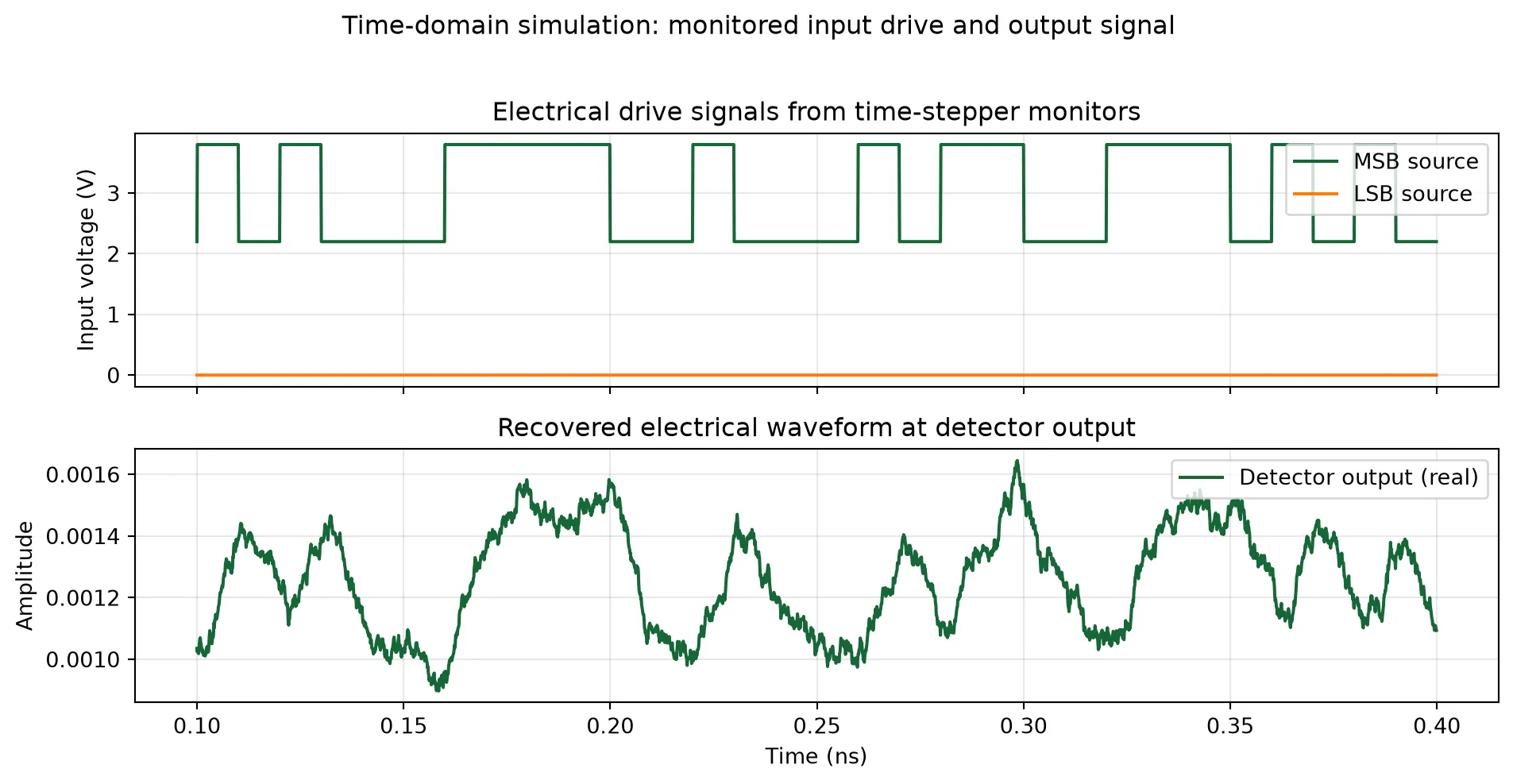

Finally, we generate an eye diagram from the recovered detector waveform to evaluate signal integrity at the target symbol rate.

The following function slices the waveform into consecutive 2T windows (with 1T shift) and overlays them on a common time axis to form the eye. We then call it with the detector output, bit rate, and time step from the simulation.

def plot_eye_diagram(optical_output_signal, bit_rate, time_step):
    """
    Plot a 2T eye diagram by slicing a uniformly sampled waveform into
    consecutive 1T-shifted windows and overlaying them on a common time axis.
    """
    # Compute sampling frequency from the time step
    Fs = 1 / time_step  # sampling frequency
    samples_per_bit = int(0.5 + Fs / bit_rate)

    # Calculate window parameters
    samples_per_window = 2 * samples_per_bit  # 2T window
    start_index = samples_per_window  # Skip initial transients

    # Calculate number of windows
    num_windows = (
        len(optical_output_signal)
        - start_index
        - (samples_per_window - samples_per_bit)
    ) // samples_per_bit
    if num_windows <= 0:
        raise ValueError("Output signal is too short to generate eye diagram.")

    # Extract signal segments for the eye diagram
    parts = []
    for k in range(num_windows):
        idx_start = start_index + k * samples_per_bit
        idx_end = idx_start + samples_per_window
        part = optical_output_signal[idx_start:idx_end]
        parts.append(part)

    parts = np.array(parts).T  # Transpose for time on x-axis

    # Time vector for plotting (centered around 0, in nanoseconds)
    t = (np.arange(samples_per_window) - samples_per_bit) * time_step * 1e12

    # Plotting
    fig, ax = plt.subplots(1, 1, tight_layout=True)
    ax.plot(t, parts, color="yellow", alpha=0.1)
    ax.set(
        xlabel="Time (ps)",
        ylabel="Detector output amplitude",
        facecolor="k",
        xlim=(t[0], t[-1]),
    )
    ax.set_title("Eye diagram (2T window, detector output)")
    ax.grid(ls=":")

plot_eye_diagram(np.real(output_signal), f_m, time_step)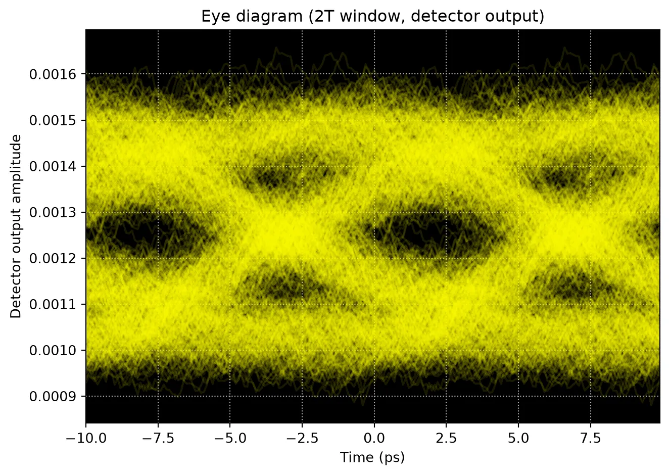

Summary and conclusion

This notebook demonstrated a compact modeling workflow for a two-segment silicon microring modulator:

1. Waveguide and coupler: We used an analytical waveguide model and replaced the full-wave directional coupler S-matrix with a compact DirectionalCouplerModel to gain speed and to add loss and modulation in a controlled way later.

2. Microring assembly: We built the MRM from passive and active segments using AnalyticWaveguideModel with PhaseModTimeStepper for electro-optic phase modulation, and validated resonance and voltage tuning in the frequency domain.

3. Time-domain testbench: We assembled a netlist with electrical drive sources (pfa.signal_source), a pfa.cw_laser for the optical input, and a pfa.photodiode for the receiver, then ran a time-domain simulation and plotted both the input voltage and the recovered electrical output. The eye diagram illustrated signal integrity at the target symbol rate.

PhotonForge APIs used

API	Purpose
AnalyticWaveguideModel	Passive and active waveguide segments with $n_\mathrm{eff}$, $n_g$, loss, $V_\pi L$, RC bandwidth
DirectionalCouplerModel	Compact bus–ring coupling (replacing full-wave S-matrix)
PhaseModTimeStepper	Voltage-dependent phase and loss in time domain
pfa.signal_source	PRBS trapezoid electrical drive
pfa.cw_laser	CW optical source
pfa.photodiode	Optical-to-electrical conversion with bandwidth and noise
component_from_netlist	Assembly of composite circuit from instances and connections