Series Push-Pull Mach-Zehnder Modulator with Slow-Wave T-Rail Electrodes
This notebook simulates a silicon-photonic carrier-depletion Mach-Zehnder modulator (MZM) using slow-wave coplanar-strip (CPS) electrodes with periodic T-shaped extensions, and connects the RF electromagnetic simulation to a time-domain optical circuit simulation. The full workflow stays in PhotonForge: the technology stack, the parametric component, the RF S-matrix solve, and the time-domain MZM circuit.
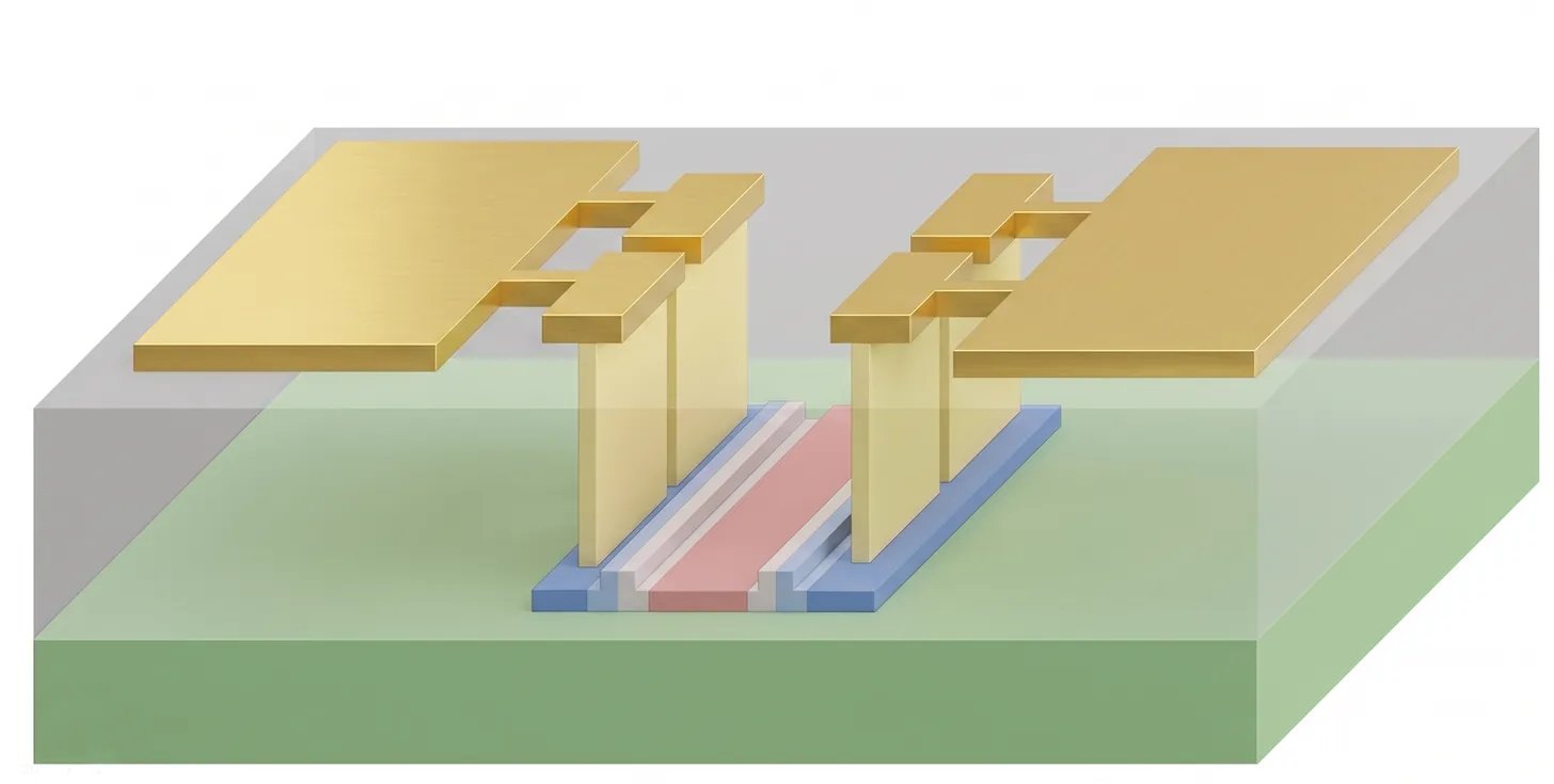
The simulated device is a series push-pull (SPP) traveling-wave MZM based on a 4-mm-long phase shifter loaded with a periodically-segmented lateral p-n junction. The two diodes of the SPP configuration are connected in series across the CPS rails, so each diode sees half of the RF voltage; the bias does not drop on the termination, eliminating the static power consumption typical of single- or dual-drive designs.
The simulation flow has three main stages:
-
3D RF electromagnetic simulation with the p-n junction modeled in-place. The slow-wave CPS electrode is built as a PhotonForge component with a Tidy3D model, and the p-n junction is added as a single lumped RLC element that bridges the two T-cap VIAs over the entire segmented region. After ABCD de-embedding of the two unloaded feed lines, the characteristic impedance Z₀, microwave effective index n_µ, and propagation loss α of the segmented section are the loaded line characteristics directly. We compare these against published reference values.
-
Frequency-domain EO S21 calculation using the analytical traveling-wave modulator response (loss + velocity mismatch + impedance mismatch), multiplied by an additional lumped RLC junction-voltage-division factor that accounts for the intrinsic R–C of the junction and the parasitic L.
-
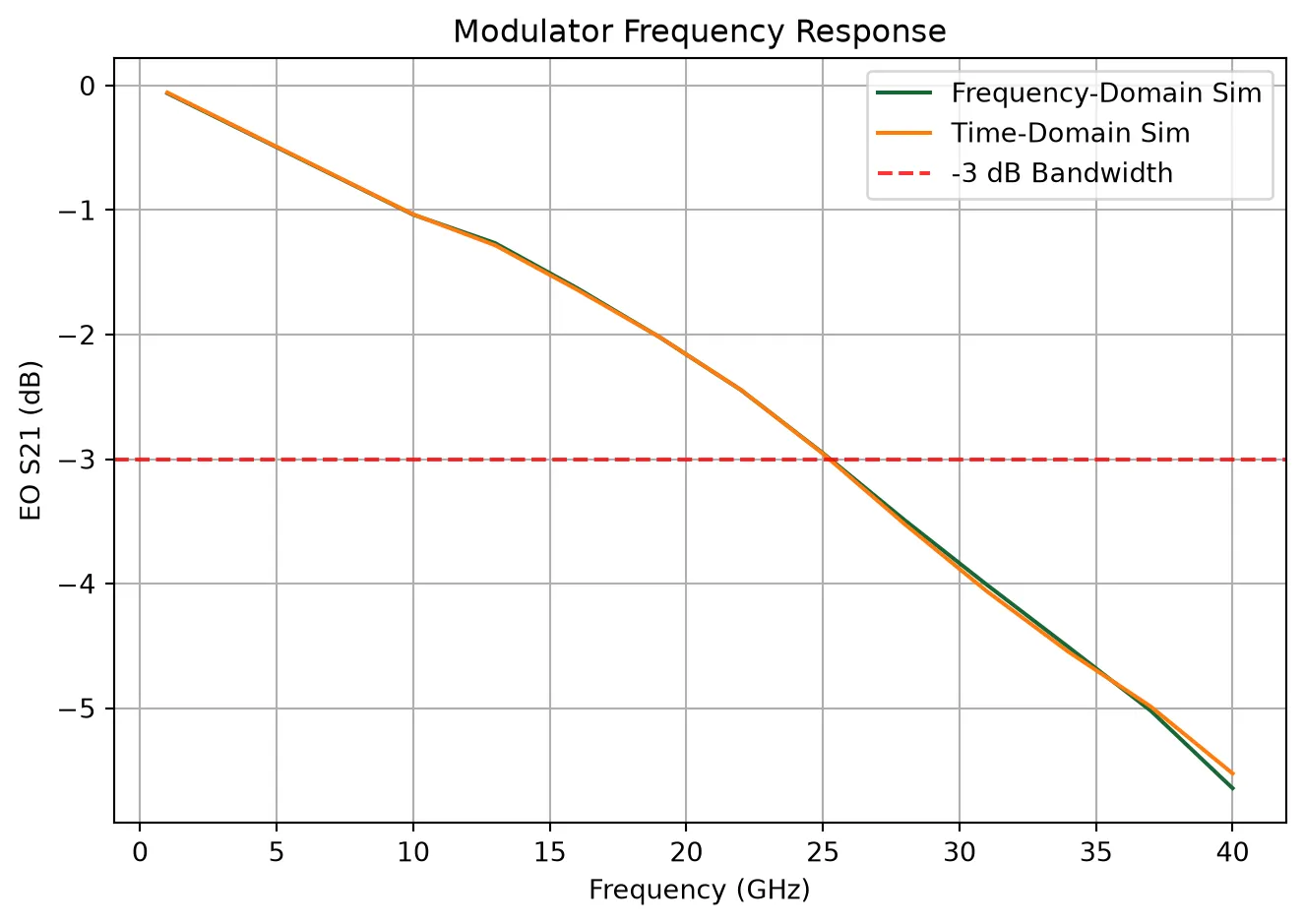
Time-domain MZM circuit simulation in PhotonForge. The full balanced MZM (laser → splitter → thermal phase tuners → push-pull EO modulator arms with RC/RLC junction filters → combiner) is built from analytic waveguide and time-stepper models, and used to verify quadrature operation, compute the optical extinction ratio, and reproduce the EO bandwidth measured in the frequency-domain analysis.
The electrical and physical parameters of the device (lateral p-n junction, modulator V_πL, propagation loss vs. bias, slow-wave T-rail geometry) follow the design described in
Reference:
- Zhuang, Dongwei, et al. “Equivalent circuit model of the carrier-depletion-based push-pull silicon optical modulators with T-rail slow wave electrodes.” IEEE Photonics Journal, 2024 16 (4), 1-9.doi: 10.1109/JPHOT.2024.3427830
- Patel, David, et al. “Design, analysis, and transmission system performance of a 41 GHz silicon photonic modulator.” Optics express, 2015 23 (11), 14263-14287, doi: 10.1364/OE.23.014263.
import matplotlib.pyplot as pltimport numpy as npimport photonforge as pfimport photonforge.abstract as pfaimport tidy3d as tdimport tidy3d.rf as rfimport tidy3d.web as webfrom photonforge.live_viewer import LiveViewer
td.config.logging.level = "ERROR"
Device parameters
Section titled “Device parameters”The modulator’s electro-optic parameters (V_πL and propagation loss) are given as a function of bias voltage from a charge-transport simulation. target_v selects the operating bias point used throughout the simulation; here we use 0 V (forward edge of the depletion regime).
The lateral p-n junction is operated in series push-pull (SPP) configuration: the two diodes (one per MZM arm) are connected in series across the CPS rails, so the line sees their series combination as a single shunt load. This halves the effective junction capacitance and doubles the effective resistance compared to a single diode, hence c_pn / 2 and r_pn × 2 below. The 4 mm length corresponds to the active phase-shifting region of the loaded line.
# Modulator properties obtained from charge simulationtarget_v = 0.0voltage_pp = 1.0  # Peak-to-peak voltage on each diodevoltages = np.linspace(-0.5, 1.0, 7)  # Reverse bias voltagesarg_v = np.argmin(np.abs(voltages - target_v))vpiL = np.array([0.85, 0.97, 1.18, 1.35, 1.51, 1.65, 1.77])modulator_loss_dB_cm = np.array([10.40, 9.99, 9.66, 9.38, 9.14, 8.91, 8.70])
# Modulator length (active phase shifter, used for EO/time-domain)length = 4000
# Junction capacitance and resistance at 0V bias:# Series push-pull (two diodes in series) -> c_pn/2, r_pn*2c_pn = 3.0136e-10 / 2r_pn = 0.0062 * 2  # in Ω·m
# RF source/load impedancez_s = 50.0z_l = 50.0
# Optical waveguide propertiesn_eff_opt = 2.56n_group_opt = 3.88wvl_um = 1.55
We sweep the RF analysis from 10 GHz to 40 GHz. This range covers the band relevant for high-speed datacom modulators (target ≥ 25 GHz EO bandwidth) and stays below the Bragg cutoff of the periodic T-rail structure.
# Frequency rangef_min, f_max = (10e9, 40e9)f0 = (f_min + f_max) / 2n_freqs = 11freqs = np.linspace(f_min, f_max, n_freqs)Slow-wave CPS geometry parameters
The slow-wave CPS consists of an n_periods-long segmented section of period period = cap_length + inter_cap_gap, flanked by two unloaded CPS launch pads of length port_offset. The two mode ports sit at the outer edge of these pads, a distance port_offset away from the segmented region, so the segmented section can later be characterized in isolation by ABCD de-embedding of the two feed lines.
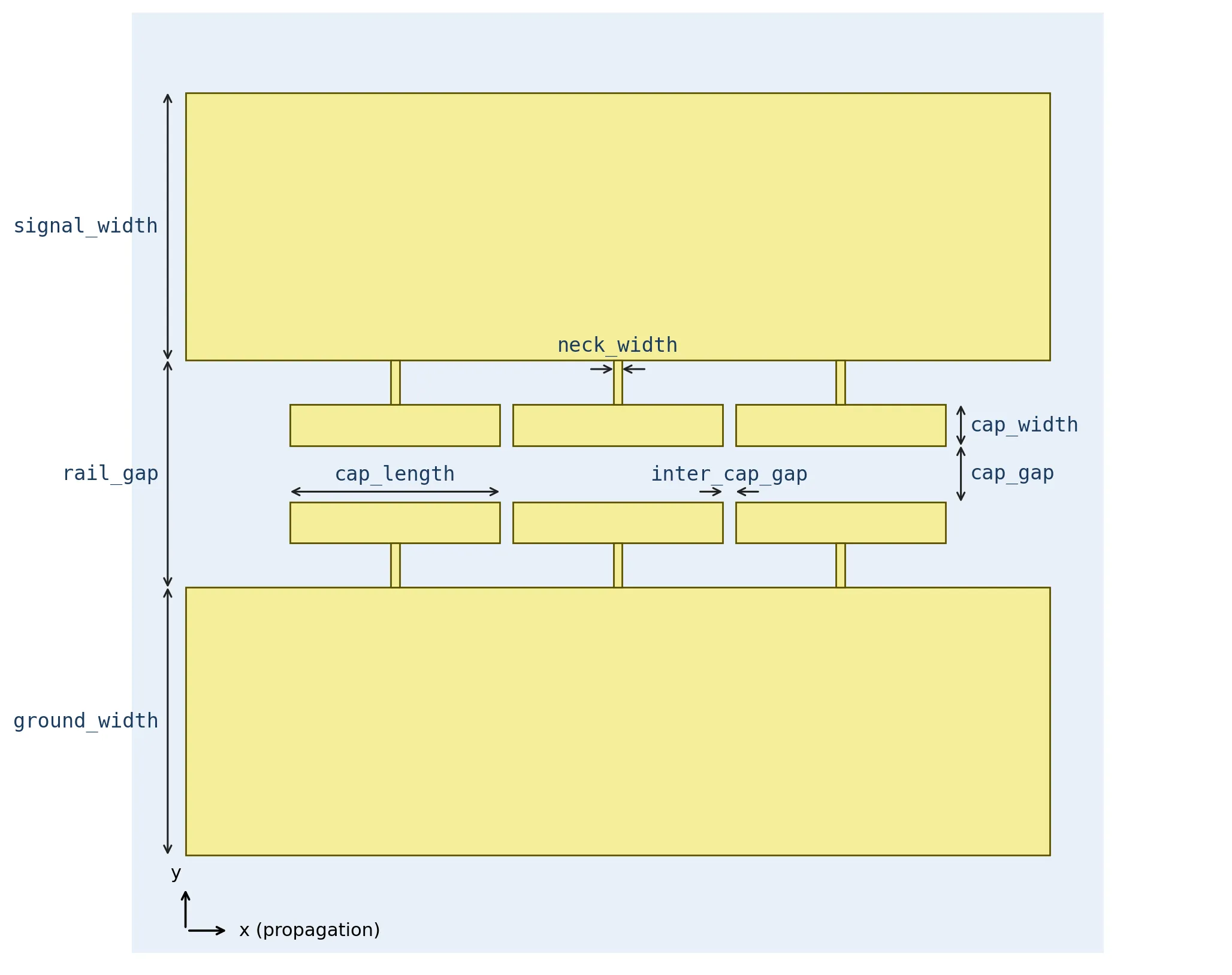
port_offset is set to 1% of the longest RF wavelength in the band, snapped to the PhotonForge grid - enough margin for the port mode to settle before reaching the segmented region.
# Top-down design parameters (μm) - Zhuang 2024 Sec III + Fig 8 captionsignal_width = 120.0  # signal CPS rail widthground_width = 120.0  # ground CPS rail widthrail_gap = 51.0  # gap between signal and ground rails (unloaded CPS)cap_gap = 12.6  # gap between opposing T-cap inner edgescap_length = 47.0  # T-cap length along x (loaded section)inter_cap_gap = 3.0  # gap between successive caps along xcap_width = 9.2  # cap thickness in y (paper "g")neck_width = 2.0  # T-rail neck width along xvia_width = 2.0  # VIA rectangle width (along y) inside each T-capvia_inset = 0.8  # VIA inset from cap inner edge (along y)slab_thickness = 0.090  # silicon slab thickness (also bottom of VIA layer)
# Segmented sectionn_periods = 20period = cap_length + inter_cap_gapl_active = n_periods * period
# Wave-port placement: 1% of the longest RF wavelength, snapped to PF gridport_offset = pf.snap_to_grid(0.01 * td.C_0 / f_min)x_port = l_active / 2.0 + port_offsetl_eff = 2 * x_port
print(f"Active region : {l_active:.1f} μm  ({n_periods} periods)")print(f"Port offset   : {port_offset:.1f} μm")print(f"L (port-port) : {l_eff:.1f} μm")
Active region : 1000.0 μm (20 periods)Port offset : 299.8 μmL (port-port) : 1599.6 μmTechnology
Section titled “Technology”A single factory make_technology(...) returns the full PhotonForge technology: layer table, materials, and extrusion stack. Layer thicknesses and every medium (substrate, oxide, silicon, metal) are exposed as keyword arguments.
@pf.parametric_technologydef make_technology(    *,    name: str = "Zhuang2024_TSWE",    version: str = "0.1",    box_thickness: float = 2.0,    slab_thickness: float = 0.090,    rib_thickness: float = 0.220,    clad_thickness: float = 1.5,    metal_thickness: float = 2.0,    metal: dict = {        "optical": td.material_library["Al"]["RakicLorentzDrude1998"],        "electrical": td.LossyMetalMedium(            conductivity=35.0,  # S/μm (= 3.5×10⁷ S/m)            frequency_range=(f_min, f_max),        ),    },    substrate: dict = {        "optical": td.material_library["cSi"]["Li1993_293K"],        "electrical": td.Medium(            permittivity=11.7,            conductivity=0.133e-6,  # S/μm, high-resistivity Si            name="Si_substrate_lossy",        ),    },    sio2: dict = {        "optical": td.material_library["SiO2"]["Horiba"],        "electrical": td.Medium(permittivity=3.9, name="SiO2_RF"),    },    si: dict = {        "optical": td.material_library["cSi"]["Li1993_293K"],        "electrical": td.Medium(permittivity=11.7, name="Si_DC"),    },    background: td.AbstractMedium = td.Medium(permittivity=1.0, name="Air"),) -> pf.Technology:    """Build the Zhuang 2024 T-rail MZM PhotonForge technology."""    layers = {        "WG": pf.LayerSpec((1, 0), "Silicon waveguide rib", "#CCE7E6", "solid"),        "SLAB": pf.LayerSpec((2, 0), "Silicon slab (90 nm)", "#CCE7E6", "//"),        "M1": pf.LayerSpec((10, 0), "Aluminum electrode metal", "#FAF7BF", "solid"),        "VIA": pf.LayerSpec((11, 0), "Metal via to silicon", "#D4A86A", "solid"),        "OUTLINE": pf.LayerSpec((99, 0), "Floorplan outline", "#777777", "hollow"),    }
    bounds = pf.MaskSpec()  # empty mask = full simulation bounds
    extrusion_specs = [        # Substrate (will be overiden by BOX)        pf.ExtrusionSpec(bounds, substrate, (-pf.Z_INF, 0)),        # Oxide (BOX + cladding)        pf.ExtrusionSpec(            bounds, sio2, (-box_thickness, slab_thickness + clad_thickness)        ),        # Silicon rib + slab (no doped-Si extrusions - RF mode is metal-dominated here)        pf.ExtrusionSpec(            pf.MaskSpec((1, 0)) + pf.MaskSpec((2, 0)),            si,            limits=(0.0, slab_thickness),        ),        pf.ExtrusionSpec(pf.MaskSpec((1, 0)), si, limits=(0.0, rib_thickness)),        # Metal stack: via from slab top to M1 underside, then M1 plate        pf.ExtrusionSpec(            pf.MaskSpec((11, 0)),            metal,            limits=(slab_thickness, slab_thickness + clad_thickness),        ),        pf.ExtrusionSpec(            pf.MaskSpec((10, 0)),            metal,            limits=(                slab_thickness + clad_thickness,                slab_thickness + clad_thickness + metal_thickness,            ),        ),    ]
    return pf.Technology(        name,        version,        layers,        extrusion_specs,        {},  # port_specs        background_medium=background,    )
tech = make_technology(slab_thickness=slab_thickness)pf.config.default_technology = techprint("Layers:", list(tech.layers))Layers: ['M1', 'OUTLINE', 'SLAB', 'VIA', 'WG']CPS mode-port spec
Section titled “CPS mode-port spec”The two mode ports sit at the outer edges of the unloaded pad regions (plain CPS with gap rail_gap = 51 μm). The port spec defines the cross-section seen by the mode solver, the integration paths used to convert the modal field to a (V, I) pair, and the target effective index used by the mode finder.
The CPS supports two quasi-TEM modes: mode index 0 is the common mode (both rails at the same potential), and mode index 1 is the differential mode (signal and ground at opposite potential). Traveling-wave excitation uses the differential mode, so we set num_modes=2 and later select mode_index=1.
port_width = 1000port_height = 1000cs_spec = pf.PortSpec(    description="CS transmission line",    width=port_width,    limits=(-port_height / 2, port_height / 2),    num_modes=2,    target_neff=2.8,    path_profiles={        "gnd": (ground_width, (rail_gap + ground_width) / 2, "M1"),        "signal": (signal_width, -(rail_gap + signal_width) / 2, "M1"),    },    voltage_path=[        (-rail_gap / 2, 3.0),        (rail_gap / 2, 3.0),    ],    current_path=[        (ground_width + rail_gap / 2 + 1, 5.0),        (0, 5.0),        (0, 1.0),        (ground_width + rail_gap / 2 + 1, 1.0),    ],)
ax = pf.tidy3d_plot(cs_spec, frequency=freqs[0])ic = cs_spec.to_tidy3d_impedance_calculator()_ = ic.voltage_integral.plot(ax=ax, x=0)_ = ic.current_integral.plot(ax=ax, x=0)ax.set_xlim((-50, 50))ax.set_ylim((-50, 50))plt.show()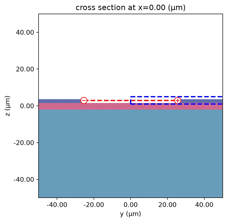
Port mode solver
Section titled “Port mode solver”Run a standalone mode solve on the unloaded CPS cross-section. We extract the two quasi-TEM modes (common at index 0, differential at index 1) and use the differential mode in everything that follows.
mode_data, z0 = pf.port_modes(cs_spec, freqs, mesh_refinement=30, impedance=True)Uploading task 'Mode-ModeSolver…'Starting task 'Mode-ModeSolver': https://tidy3d.simulation.cloud/workbench?taskId=mo-fd16828f-bfc9-499a-b795-7235e4e523e0Downloading data from 'Mode-ModeSolver'…Plot the real part of at the highest frequency for the differential mode (mode_index=1). Under the rail-gap mirror plane (x=0), is even (same sign on both sides) because the differential CPS mode has pointing across the gap.
ax = mode_data.plot_field("Ey", "real", f=freqs[-1], mode_index=1, robust=False)ax.set_xlim((-50, 50))ax.set_ylim((-50, 50))plt.show()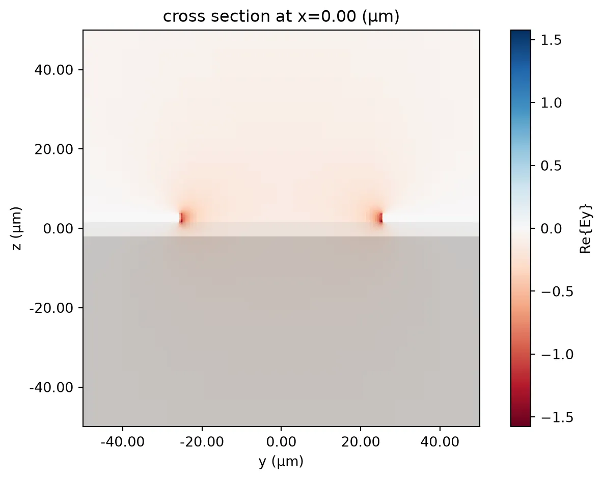
Extract the unloaded-line characteristic impedance Z₀, microwave effective index n_µ, and propagation loss α directly from the mode-solver results (differential mode).
# Gather alpha, neff from mode solver results (differential mode = index 1)z0 = ic.compute_impedance(mode_data.data).isel(mode_index=1)alpha_mode_dB_cm = mode_data.data.modes_info["loss (dB/cm)"].sel(mode_index=1)neff_mode = mode_data.data.n_eff.isel(mode_index=1)
fig, axes = plt.subplots(1, 3, figsize=(12, 3), tight_layout=True)
axes[2].plot(freqs / 1e9, z0.real, "o-", label="PhotonForge")axes[2].set_xlabel("Frequency (GHz)")axes[2].set_ylabel("Real Impedance (Ω)")axes[2].set_ylim(70, 90)
axes[1].plot(freqs / 1e9, neff_mode, "o-", label="PhotonForge")axes[1].set_xlabel("Frequency (GHz)")axes[1].set_ylabel("RF Effective Index")axes[1].set_ylim(2, 3.0)
axes[0].plot(freqs / 1e9, alpha_mode_dB_cm, "o-", label="PhotonForge")axes[0].set_xlabel("Frequency (GHz)")axes[0].set_ylabel("RF Loss (dB/cm)")plt.show()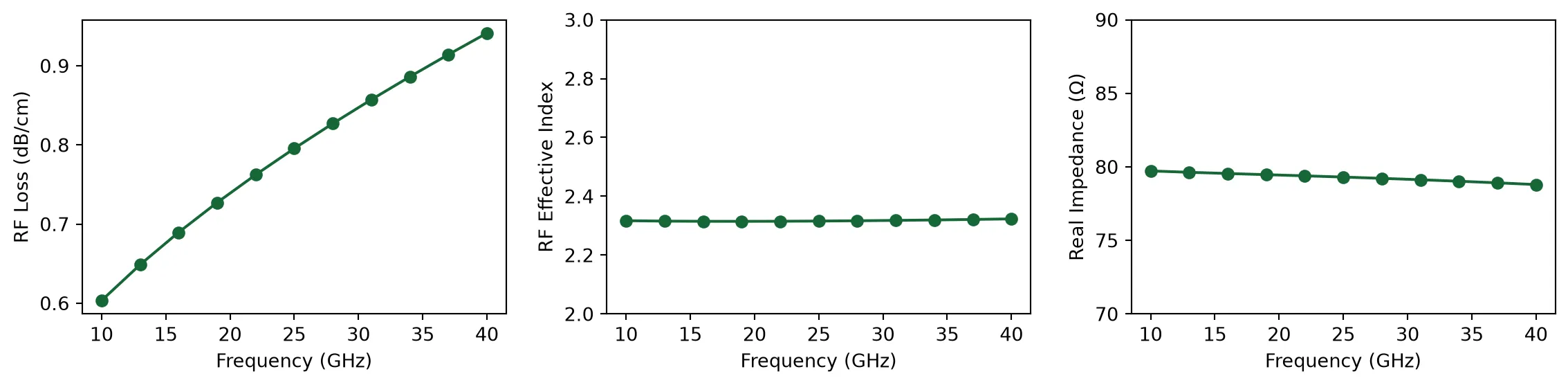
Segmented CPS component (3D analysis)
Section titled “Segmented CPS component (3D analysis)”A function tswe_with_pads(...) builds the full TSWE: continuous outer CPS rails along the whole length, plus an array of T-extensions (signal + ground neck and cap) in the central segmented section. The unloaded pads on each side carry the mode ports and are de-embedded later.
Silicon ribs and push-pull doping are intentionally not drawn here: only the metal influences the 3D RF mode at this level of analysis, and removing the 90 nm-thick rib/slab avoids forcing the auto-grid into an excessively small time step.
The PN junction is modeled as a single lumped RLC element that bridges the two T-cap VIAs over the entire segmented region. A series R–C network (with a vestigial L ≈ 0) is built from the per-unit-length r_pn and c_pn set in the device-parameters cell, integrated over the segmented length l_active, and inserted into the Tidy3D simulation that PhotonForge generates by passing simulation_updates={"lumped_elements": [pn_junction]} to the component’s Tidy3DModel. With the junction inside the FDTD, the de-embedded segmented-line characteristics in the next section are the loaded line directly.
@pf.parametric_componentdef tswe_with_pads(    *,    n_periods: int = 20,    port_offset: float = 100.0,    signal_width: float = 120.0,    ground_width: float = 120.0,    rail_gap: float = 51.0,    cap_gap: float = 12.6,    cap_length: float = 47.0,    inter_cap_gap: float = 3.0,    cap_width: float = 9.2,    neck_width: float = 2.0,    via_width: float = 2.0,    via_inset: float = 0.8,    slab_thickness: float = 0.090,    r_pn: float = 0.0124,    c_pn: float = 1.5068e-10,    technology: pf.Technology | None = None,) -> pf.Component:    """Segmented T-rail CPS flanked by two unloaded launch pads (M1 only).
    The central segmented section has `n_periods` T-extensions of period    `cap_length + inter_cap_gap`. Each side has a length-`port_offset`    plain CPS pad with gap `rail_gap`, sized to host a mode port at its    outer edge. Inside each T-cap, a VIA rectangle of width `via_width`    is placed `via_inset` away from the cap's inner edge.
    The lateral p-n junction is added to the Tidy3D simulation as a single    lumped RLC element bridging the two T-cap VIAs over the segmented    region, via `Tidy3DModel.simulation_updates`. `r_pn` (Ω·m) and    `c_pn` (F/m) are the series push-pull values.    """    period = cap_length + inter_cap_gap    stem_len = (rail_gap - cap_gap) / 2.0 - cap_width    l_active = n_periods * period    l_total = l_active + 2 * port_offset
    c = pf.Component(        name=f"TSWE_{n_periods}p_pad{port_offset:.0f}",        technology=technology,    )    x0_t, xr_t = -l_total / 2.0, +l_total / 2.0    x0_a = -l_active / 2.0
    # Continuous outer CPS rails along whole length    c.add(        "M1",        pf.Rectangle((x0_t, +rail_gap / 2), (xr_t, +rail_gap / 2 + signal_width)),        pf.Rectangle((x0_t, -rail_gap / 2 - ground_width), (xr_t, -rail_gap / 2)),    )
    # Per-period T-cell metal + VIA: signal/ground necks, caps, and vias    via_y_min = cap_gap / 2 + via_inset    via_y_max = via_y_min + via_width    for k in range(n_periods):        x_center = x0_a + (k + 0.5) * period        cap_x_left = x_center - cap_length / 2.0        cap_x_right = x_center + cap_length / 2.0        c.add(            "M1",            # signal neck            pf.Rectangle(                (x_center - neck_width / 2, +cap_gap / 2 + cap_width),                (x_center + neck_width / 2, +cap_gap / 2 + cap_width + stem_len),            ),            # signal cap            pf.Rectangle(                (cap_x_left, +cap_gap / 2),                (cap_x_right, +cap_gap / 2 + cap_width),            ),            # ground neck            pf.Rectangle(                (x_center - neck_width / 2, -cap_gap / 2 - cap_width - stem_len),                (x_center + neck_width / 2, -cap_gap / 2 - cap_width),            ),            # ground cap            pf.Rectangle(                (cap_x_left, -cap_gap / 2 - cap_width),                (cap_x_right, -cap_gap / 2),            ),        )        c.add(            "VIA",            # signal-side VIA inside the signal cap            pf.Rectangle((cap_x_left, +via_y_min), (cap_x_right, +via_y_max)),            # ground-side VIA inside the ground cap            pf.Rectangle((cap_x_left, -via_y_max), (cap_x_right, -via_y_min)),        )
        # PN junction as a single lumped RLC element bridging signal/ground VIAs.        # A tiny dummy inductance keeps the RLCNetwork valid without contributing.        l_seg_m = l_active * 1e-6        junction_network = td.rf.RLCNetwork(            resistance=r_pn / l_seg_m,            capacitance=c_pn * l_seg_m,            inductance=1e-20,            network_topology="series",        )        overlap = 0.0        pn_junction = td.LinearLumpedElement(            center=[0.0, 0.0, slab_thickness],            size=[l_active, 2 * via_y_min + 2 * overlap, 0],            voltage_axis=1,  # voltage drop in y (signal -> ground)            network=junction_network,            name="PN_junction",        )
        c.add_model(            pf.Tidy3DModel(                boundary_spec=td.BoundarySpec(                    x=td.Boundary.pml(num_layers=30),                    y=td.Boundary.pml(),                    z=td.Boundary.pml(),                ),                simulation_updates={"lumped_elements": [pn_junction]},            )        )        c.add_port(c.detect_ports([cs_spec], on_boundary="x"))
    return c
comp = tswe_with_pads( n_periods=n_periods, port_offset=port_offset, signal_width=signal_width, ground_width=ground_width, rail_gap=rail_gap, cap_gap=cap_gap, cap_length=cap_length, inter_cap_gap=inter_cap_gap, cap_width=cap_width, neck_width=neck_width, via_width=via_width, via_inset=via_inset, slab_thickness=slab_thickness, r_pn=r_pn, c_pn=c_pn, technology=tech,)
viewer = LiveViewer()viewer(comp)LiveViewer started at http://127.0.0.1:41467. Call its 'stop()' method to free the port.
Also plot a static transverse cross-section in the unloaded pad to confirm that the structure and grid are set up properly around the metal traces.
fig, ax = plt.subplots()pf.tidy3d_plot(comp, x=-75, ax=ax)ax.set_xlim([-20, 20])ax.set_ylim([-2.5, 5.0])plt.tight_layout()plt.show()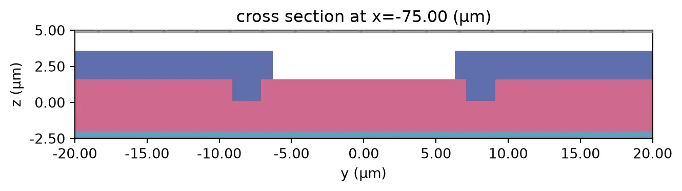
Run the 3D RF simulation
Section titled “Run the 3D RF simulation”Run the FDTD S-matrix solve through the Tidy3DModel. We restrict the excitation to E0@1 - the differential CPS mode at port E0, i.e. the second mode (index 1) at that port - since that is the only mode of physical interest for traveling-wave operation. The S-parameters between the two ports for this mode are what we feed into the de-embedding step below.
# Visual sanity check of the lumped-element placementsim = comp.active_model.get_simulations(comp, freqs)["E0@1"]sim.plot(z=slab_thickness, hlim=(-l_active / 2 - 30, l_active / 2 + 30), vlim=(-30, 30))plt.show()
s_matrix = comp.s_matrix(freqs, model_kwargs={"inputs": ["E0@1"]})_ = pf.plot_s_matrix(s_matrix, y="dB")plt.show()
s11 = s_matrix[("E0@1", "E0@1")]s21 = s_matrix[("E0@1", "E1@1")]
Uploading task 'E0@1…'Starting task 'E0@1': https://tidy3d.simulation.cloud/workbench?taskId=fdve-1080bba2-2584-4054-b05c-f58efb86a011Downloading data from 'E0@1'…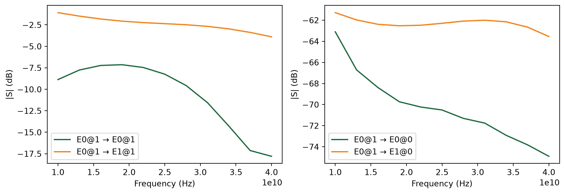
De-embedding and characterization of the segmented section
Section titled “De-embedding and characterization of the segmented section”The mode ports sit in the unloaded CPS at a port_offset distance from the segmented (T-rail) section. To recover the intrinsic propagation constant and characteristic impedance of the segmented section alone, we de-embed the two unloaded feed lines using ABCD-matrix arithmetic.
The procedure: (A) convert the full S-matrix into ABCD form, (B) build the ABCD of one unloaded feedline of length l_feed_m from the mode-solver gamma_mode and z0, (C) left- and right-multiply by the inverse feedline ABCD to strip the feeds, and (D) extract Z and γ of the segmented line directly from the de-embedded ABCD. The phase-unwrap step uses an n_eff_guess = 3.5 to resolve 2π ambiguities in β·L.
# 1. Constants and lengthsc = 299_792_458.0  # m/somega = 2 * np.pi * freqs  # rad/s
l_feed_m = port_offset * 1e-6  # one-side feedline length (m)l_seg_m = l_active * 1e-6  # segmented section length (m)
# 2. Pull arrays out of xarray containersdef _to_1d(x):    a = np.asarray(x.values if hasattr(x, "values") else x)    return a.squeeze()
# Convert loss from dB/cm to Nepers/m (alpha)alpha_mode = (alpha_mode_dB_cm * 100.0) / (20.0 * np.log10(np.e))
# Calculate beta (rad/m) from the real part of neffbeta_mode = (omega * neff_mode.values.real) / 299792458.0
# Combine into complex Gamma (1/m)gamma_mode = alpha_mode - 1j * beta_mode
gamma_feed = _to_1d(gamma_mode)z_ref_port = np.conjugate(_to_1d(z0))
num_freqs = len(freqs)z0_modulator = np.zeros(num_freqs, dtype=complex)gamma_seg = np.zeros(num_freqs, dtype=complex)
# 3. De-embed and extract per-frequencyfor i in range(num_freqs):    z0_i = z_ref_port[i]    s11_i = s11[i]    s21_i = s21[i]    g_i = gamma_feed[i]
    # --- Step A: S -> ABCD of the full DUT (reciprocal & symmetric) ---    denom = 2 * s21_i    a_tot = ((1 + s11_i) * (1 - s11_i) + s21_i**2) / denom    b_tot = z0_i * ((1 + s11_i) ** 2 - s21_i**2) / denom    c_tot = (1.0 / z0_i) * ((1 - s11_i) ** 2 - s21_i**2) / denom    d_tot = a_tot    abcd_tot = np.array([[a_tot, b_tot], [c_tot, d_tot]])
    # --- Step B: feedline ABCD ---    cgL = np.cosh(g_i * l_feed_m)    sgL = np.sinh(g_i * l_feed_m)    a_f, b_f = cgL, z0_i * sgL    c_f, d_f = sgL / z0_i, cgL
    # Inverse of a unimodular ABCD (AD - BC = 1 for a passive line)    abcd_feed_inv = np.array([[d_f, -b_f], [-c_f, a_f]])
    # --- Step C: de-embed one feedline from each side ---    abcd_seg = abcd_feed_inv @ abcd_tot @ abcd_feed_inv
    a_seg = abcd_seg[0, 0]    b_seg = abcd_seg[0, 1]    c_seg = abcd_seg[1, 0]
    # --- Step D: characteristic impedance and propagation constant ---    z_i = np.sqrt(b_seg / c_seg)    if np.real(z_i) < 0:        z_i = -z_i    z0_modulator[i] = z_i
    root = np.sqrt(a_seg**2 - 1 + 0j)    t1, t2 = a_seg + root, a_seg - root    # Pick the passive (forward-propagating) branch: |T| < 1 for a lossy line.    t = t1 if np.abs(t1) <= 1 else t2    gamma_seg[i] = -np.log(t) / l_seg_m
# 4. Metricsalpha_np_m = np.real(gamma_seg)  # Np/malpha_db_cm = alpha_np_m * 8.686 / 100.0  # dB/cm
# Phase unwrap with a physical n_eff referencen_eff_guess = 3.5beta_L_raw = np.angle(np.exp(-gamma_seg * l_seg_m))expected = n_eff_guess * omega / c * l_seg_mn_wraps = np.round((expected - beta_L_raw) / (2 * np.pi)).astype(int)beta_L_unwrp = beta_L_raw + 2 * np.pi * n_wrapsbeta_rad_m = beta_L_unwrp / l_seg_mn_eff_rf = beta_rad_m * c / omega
Reference data: loaded line
Section titled “Reference data: loaded line”Loss, microwave effective index, and characteristic impedance of the loaded slow-wave CPS line as published in [1]. These values serve as the validation target for our simulated loaded-line characteristics in the next cell.
f_ref_1 = np.array(    [        10.034843205574914,        15.470383275261321,        19.372822299651567,        22.020905923344948,        24.52961672473867,        27.317073170731703,        30.522648083623693,        34.98257839721255,        40.00000000000001,    ])
alpha_ref = np.array(    [        45.714285714285744,        80.95238095238098,        120.95238095238099,        157.1428571428572,        203.80952380952385,        255.23809523809527,        297.1428571428572,        325.71428571428584,        337.1428571428572,    ])
f_ref_2 = np.array([9.895470383275264, 19.930313588850172, 30.104529616724747, 40.0])n_eff_ref = np.array(    [3.8571428571428577, 3.8476190476190477, 3.823809523809524, 3.804761904761905])
f_ref_3 = np.array(    [9.853894887569824, 19.92257677802847, 29.997585727486918, 40.07126266452434])z_ref = np.array(    [48.13393384893314, 48.26780109724523, 47.72309126782608, 47.32123977056086])
Compare the simulated loaded-line loss, microwave effective index, and real characteristic impedance against the reference measurements.
fig, axes = plt.subplots(1, 3, figsize=(12, 4), tight_layout=True)
axes[0].plot(freqs / 1e9, alpha_db_cm / 0.08686, "o-", label="PhotonForge")axes[0].plot(f_ref_1, alpha_ref, "s--", label="Ref: Zhuang 2024", alpha=0.7)axes[0].set_xlabel("Frequency (GHz)")axes[0].set_ylabel("Loss (Neper/m)")axes[0].legend()
axes[1].plot(freqs / 1e9, n_eff_rf, "o-", label="PhotonForge")axes[1].plot(f_ref_2, n_eff_ref, "s--", label="Ref: Zhuang 2024", alpha=0.7)axes[1].set_xlabel("Frequency (GHz)")axes[1].set_ylabel("RF Effective Index")axes[1].set_ylim((3, 5))axes[1].legend()
axes[2].plot(freqs / 1e9, np.real(z0_modulator), "o-", label="PhotonForge")axes[2].plot(f_ref_3, z_ref, "s--", label="Ref: Zhuang 2024", alpha=0.7)axes[2].set_xlabel("Frequency (GHz)")axes[2].set_ylabel("Real Impedance (Ω)")axes[2].set_ylim((40, 60))axes[2].legend()
plt.show()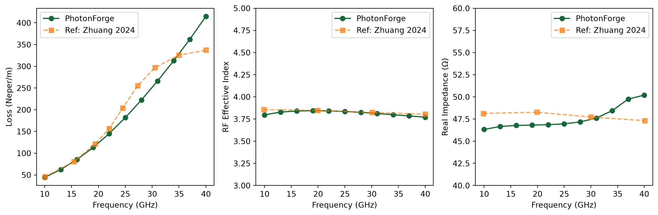
EO S-Parameters
Section titled “EO S-Parameters”Compute the electro-optic S21 of the traveling-wave modulator using the standard analytical model that combines microwave loss, velocity mismatch, and impedance mismatch. The result is then multiplied by an additional lumped RLC factor that captures the junction’s intrinsic voltage division (the fraction of the line voltage that drops across the depletion capacitance) before being compared against measured EO S21 data.
def eo_s21(rf_loss, rf_frequencies, n_rf, n_group, length, z_load, z_source, z0):    """EO S21 of a traveling-wave modulator (output phase change normalized to DC).
    rf_loss in dB/μm; rf_frequencies in Hz; length in μm; impedances in Ω.    """    c = pf.C_0    omega = 2 * np.pi * rf_frequencies    alpha_np_um = rf_loss / 8.686
    gamma_m = alpha_np_um + 1j * (omega / c) * n_rf
    F_plus = (1 - np.exp(gamma_m * length - 1j * (omega / c) * n_group * length)) / (        gamma_m * length - 1j * (omega / c) * n_group * length    )    F_minus = (1 - np.exp(-gamma_m * length - 1j * (omega / c) * n_group * length)) / (        -gamma_m * length - 1j * (omega / c) * n_group * length    )
    z_in = (        z0        * (z_load + z0 * np.tanh(gamma_m * length))        / (z0 + z_load * np.tanh(gamma_m * length))    )
    return -(        (2 * z_in / (z_in + z_source))        * ((z_load + z0) * F_plus + (z_load - z0) * F_minus)        / (            (z_load + z0) * np.exp(gamma_m * length)            + (z_load - z0) * np.exp(-gamma_m * length)        )    )
Measured EO S21 at 0 V bias, extracted from Fig. 9(b) of [2]. Used as the validation target for the analytical EO response.
f_meas_GHz = np.array(    [        0.02,        0.72,        1.85,        2.80,        3.62,        4.76,        5.46,        6.78,        8.11,        9.00,        9.82,        10.64,        11.33,        12.09,        13.35,        14.80,        16.45,        17.71,        18.72,        19.92,        21.30,        22.82,        23.96,        25.03,        26.93,        27.93,        28.50,        29.64,        30.46,        31.34,        32.29,        33.30,        34.75,        35.76,        35.76,        37.03,        38.10,        39.29,        40.11,        41.88,        42.77,        43.78,        45.17,        45.42,    ])
eo_s21_meas = np.array(    [        -0.56,        0.11,        -0.16,        -0.45,        -0.40,        -0.24,        -0.21,        -0.29,        -0.11,        -0.11,        -0.34,        -0.64,        -0.82,        -0.98,        -1.30,        -1.17,        -0.90,        -1.17,        -1.59,        -1.96,        -2.20,        -2.36,        -2.28,        -2.39,        -2.57,        -3.10,        -3.53,        -3.58,        -4.01,        -4.35,        -4.22,        -4.27,        -4.24,        -4.43,        -4.43,        -4.14,        -4.99,        -5.65,        -5.73,        -6.13,        -5.97,        -6.29,        -6.07,        -6.37,    ])
Assemble the full frequency-domain EO response in three pieces:
- Frequency extrapolation down to 1 GHz so the EO response can be normalized to a low-frequency limit. At 1 GHz the junction still loads the line strongly (junction susceptance is comparable to its 10 GHz value), so we replicate the 10 GHz values of n_eff, Z₀, and α for the 1 GHz point.
- Junction RLC voltage divider -
h_rlc = 1 / (1 - ω²LC + jωRC)with lumpedr_tot = r_pn / L,c_tot = c_pn · L, and an empirical parasitic inductancel_parasitic = 5 pH. This captures the fact that not all of the line-side voltage drops across the depletion capacitance. - Traveling-wave EO transfer function
h_twfrom the analytical model, multiplied byh_rlcto give the total EO S21.
The result is overlaid on the measured 0 V data; agreement validates both the loaded-line extraction and the choice of l_parasitic.
# 0. Extrapolate into new arrays to include 1 GHz at the beginningfreqs_ext = np.insert(freqs, 0, 1e9)n_eff_rf_ext = np.insert(n_eff_rf, 0, n_eff_rf[0])z0_modulator_ext = np.insert(z0_modulator, 0, z0_modulator[0])# Two-point power-law extrapolation alpha = A * f^n (always positive,# matches the data curvature better than linear).alpha_n = np.log(alpha_db_cm[1] / alpha_db_cm[0]) / np.log(freqs[1] / freqs[0])alpha_at_1ghz = alpha_db_cm[0] * (1e9 / freqs[0]) ** alpha_nalpha_db_cm_ext = np.insert(alpha_db_cm, 0, alpha_at_1ghz)
omega_ext = 2 * np.pi * freqs_ext
# 1. Empirical port-to-junction parasitic inductance and total junction R, Cl_parasitic = 5e-12c_tot = c_pn * length * 1e-6r_tot = r_pn / (length * 1e-6)
# 2. RLC frequency response: H(w) = 1 / (1 - w^2*L*C + j*w*R*C)h_rlc = 1 / (    (1 - (omega_ext**2) * l_parasitic * c_tot) + 1j * omega_ext * r_tot * c_tot)
# 3. Traveling Wave EO S21h_tw = eo_s21(    alpha_db_cm_ext * 1e-4,    freqs_ext,    n_eff_rf_ext,    n_group_opt,    length,    z_l,    z_s,    z0_modulator_ext,)
# 4. Total responseh_total = h_tw * h_rlc
# 5. Plotplt.figure()plt.plot(    freqs_ext * 1e-9,    20 * np.log10(np.abs(h_total)),    label="Total Response (TW + RLC)",)plt.plot(    freqs_ext * 1e-9, 20 * np.log10(np.abs(h_tw)), "--", label="Traveling Wave Only")plt.plot(f_meas_GHz, eo_s21_meas, "s--", label="Measurement", alpha=0.7)plt.xlabel("Frequency (GHz)")plt.ylabel("EO S21 (dB)")plt.title("Modulator Frequency Response")plt.grid(True)plt.legend()plt.tight_layout()plt.show()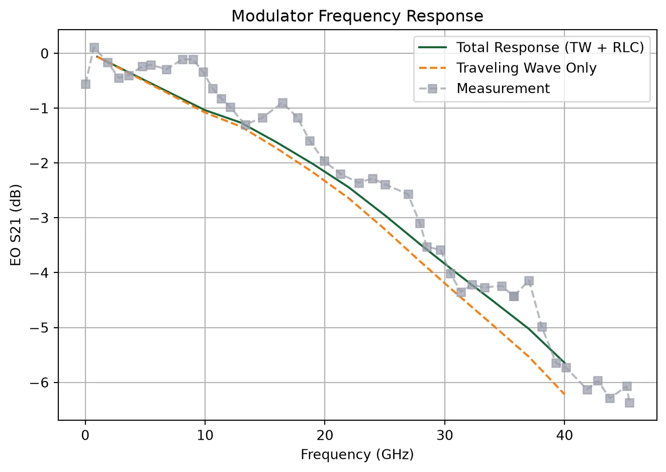
Time-domain MZM circuit
Section titled “Time-domain MZM circuit”Build the MZM as a PhotonForge circuit (virtual ports): laser → splitter → thermal arms → EO arms (with RC LPF and push-pull drive) → combiner. Uses vpiL, modulator_loss_dB_cm, n_eff_opt, n_group_opt, length, n_eff_rf, alpha_db_cm, and f_cutoff from above.
Phase Model Fitting
Section titled “Phase Model Fitting”Fit a polynomial to the extracted VπL(V) curve so it can be used in time-domain circuit simulations.
vpiL_um = vpiL * 10000.0  # convert V·cm -> V·µminv_vpiL_um = 1.0 / vpiL_um  # 1/(V·µm)
# polyfit returns highest-order first: [c2, c1, c0] for c0 + c1*V + c2*V^2c2, c1, c0 = np.polyfit(voltages, inv_vpiL_um, 2)
# Map polynomial coefficients back to the physical parametersv_piL_linear = 1.0 / c0  # V·µm  (small-signal VpiL at V=0)k2_fit = c1 * np.pi / 2.0  # rad/(V^2·µm)k3_fit = c2 * np.pi / 3.0  # rad/(V^3·µm)
def calculate_vpiL_from_fit(V, v_piL_linear, k2, k3):    """v_piL_linear in V·µm, k2 in rad/(V^2·µm), k3 in rad/(V^3·µm); returns V·cm."""    dphi_dV = (np.pi / v_piL_linear) + 2.0 * k2 * V + 3.0 * k3 * V**2    vpiL_um = np.pi / dphi_dV    return vpiL_um / 10000.0
vpiL_fit_cm = calculate_vpiL_from_fit(voltages, v_piL_linear, k2_fit, k3_fit)
plt.figure()plt.plot(voltages, vpiL, "o", label="Original Simulation Data", markersize=8)plt.plot(voltages, vpiL_fit_cm, "-", label="Fitted Model", linewidth=2)plt.xlabel("Applied Voltage (V)")plt.ylabel(r"$V_\pi L$ (V$\cdot$cm)")plt.title(r"$V_\pi L$ vs Voltage")plt.legend()plt.grid(True, linestyle="--", alpha=0.7)plt.tight_layout()plt.show()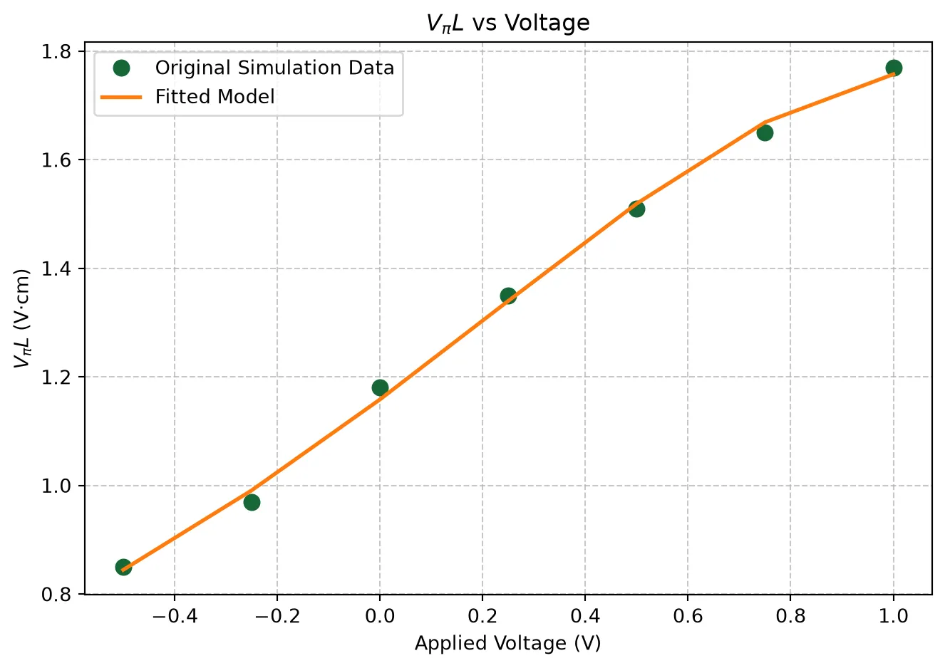
Set up the time-domain simulation parameters: the RC junction cutoff f_cutoff, the average optical propagation loss, the optical carrier frequency, the thermal-arm quadrature bias, and PhotonForge Interpolator objects for the RF line characteristics. Then define the parametric MZM testbench create_mzm.
Junction filter: RC approximation
Section titled “Junction filter: RC approximation”The junction voltage division is approximated by a first-order RC low-pass filter implemented via PhotonForge’s FilterTimeStepper with family='rc':
Approximation: dropping the parasitic inductance
Section titled “Approximation: dropping the parasitic inductance”The full second-order junction model is
We drop the term, which is justified when , i.e., . Below this section we will use the simpler RC model; the full RLC version with a digital IIR is implemented further down for completeness.
# --- Time-domain / circuit params ---f_cutoff = 1 / (2 * np.pi * r_tot * c_tot)loss_dB_um = np.mean(modulator_loss_dB_cm) * 1e-4f_c = td.C_0 / wvl_um  # Hzthermal_length_um = 100# Thermal arms: bias MZM at quadrature (π/2 phase between arms)dn_dT = 1e-4t0_k = 293.0delta_t_k_quad = (np.pi / 2) * wvl_um / (2 * np.pi * thermal_length_um * dn_dT)
# Creating frequency-dependent parametersn_rf_freqs = pf.Interpolator(freqs_ext, n_eff_rf_ext)z0_freqs = pf.Interpolator(freqs_ext, z0_modulator_ext)# Set extrapolation = "constant"# This is very important to avoid extrapolate non-physically large numbers at very high frequencies in time domain simulationalpha_db_um_freqs = pf.Interpolator(    freqs_ext, alpha_db_cm_ext * 1e-4, extrapolation="constant")
@pf.parametric_componentdef create_mzm(    v_pp_drive=voltage_pp,    length=length,    thermal_delta_t_k=delta_t_k_quad,    signal_freq=1e9,):
    opt_vir = pf.virtual_port_spec(classification="optical")    elec_vir = pf.virtual_port_spec(classification="electrical")
    # Laser    laser = pfa.cw_laser(power=1e-3)
    # Splitters / combiner    splitter = pfa.y_splitter()    combiner = pfa.y_splitter()
    # Waveguides with heaters for adjusting the bias point    therm1 = pfa.straight(        n_eff=n_eff_opt,        length=thermal_length_um,        propagation_loss=0.0,        dn_dT=dn_dT,        temperature=t0_k,    )    therm2 = pfa.straight(        n_eff=n_eff_opt,        length=thermal_length_um,        propagation_loss=0.0,        dn_dT=dn_dT,        temperature=t0_k + thermal_delta_t_k,    )
    # First arm traveling wave modulator    mod_model_1 = pf.AnalyticWaveguideModel(        n_eff=n_eff_opt, length=length, propagation_loss=loss_dB_um, n_group=n_group_opt    )    mod_model_1.time_stepper = pf.TerminatedModTimeStepper(        v_piL=v_piL_linear,        length=length,        n_eff=n_eff_opt,        n_group=n_group_opt,        n_rf=n_rf_freqs,        propagation_loss=loss_dB_um,        rf_propagation_loss=alpha_db_um_freqs,        z0=z0_freqs,        z_load=z_l,        z_source=z_s,        k2=k2_fit,        k3=k3_fit,    )    mod1 = mod_model_1.black_box_component(opt_vir, name="Mod1")    mod1.add_port(pf.Port((0.5, 0.5), -90, spec=elec_vir), "E0")
    # Second arm traveling wave modulator    mod_model_2 = pf.AnalyticWaveguideModel(        n_eff=n_eff_opt, length=length, propagation_loss=loss_dB_um, n_group=n_group_opt    )    mod_model_2.time_stepper = pf.TerminatedModTimeStepper(        v_piL=v_piL_linear,        length=length,        n_eff=n_eff_opt,        n_group=n_group_opt,        n_rf=n_rf_freqs,        propagation_loss=loss_dB_um,        rf_propagation_loss=alpha_db_um_freqs,        z0=z0_freqs,        z_load=z_l,        z_source=z_s,        k2=k2_fit,        k3=k3_fit,    )    mod2 = mod_model_2.black_box_component(opt_vir, name="Mod2")    mod2.add_port(pf.Port((0.5, 0.5), -90, spec=elec_vir), "E0")
    # Electrical sources (push-pull at target_v)    amplitude_src = (v_pp_drive / 2) / np.sqrt(z_s)
    src = pfa.signal_source(        frequency=signal_freq,        amplitude=amplitude_src,        offset=target_v / np.sqrt(z_s),        waveform="sine",    )    src2 = pfa.signal_source(        frequency=signal_freq,        amplitude=amplitude_src,        offset=target_v / np.sqrt(z_s),        waveform="sine",        start=0.5 / signal_freq,    )
    # RC LPF at the f_cutoff computed above    lpf = pfa.filter(family="rc", shape="lp", f_cutoff=f_cutoff, order=1)    lpf2 = pfa.filter(family="rc", shape="lp", f_cutoff=f_cutoff, order=1)
    netlist = {        "name": "SISCAP_MZM_Testbench",        "instances": {            "splitter": {"component": splitter, "origin": (0, 0)},            "combiner": {"component": combiner, "origin": (11, 0)},            "therm1": {"component": therm1, "origin": (5, 1)},            "therm2": {"component": therm2, "origin": (5, -1)},            "mod1": {"component": mod1, "origin": (9, 1)},            "mod2": {"component": mod2, "origin": (9, -1)},            "laser": {"component": laser, "origin": (-2, 0)},            "src": {"component": src, "origin": (9, -1.5)},            "src2": {"component": src2, "origin": (9, 1.5)},            "lpf": {"component": lpf, "origin": (9, -1.3)},            "lpf2": {"component": lpf2, "origin": (9, 1.3)},        },        "connections": [            (("laser", "P0"), ("splitter", "P0")),            (("therm1", "P0"), ("splitter", "P1")),            (("mod1", "P0"), ("therm1", "P1")),            (("therm2", "P0"), ("splitter", "P2")),            (("mod2", "P0"), ("therm2", "P1")),            (("combiner", "P2"), ("mod1", "P1")),            (("mod2", "P1"), ("combiner", "P1")),            (("lpf", "E1"), ("mod1", "E0")),            (("lpf2", "E1"), ("mod2", "E0")),            (("src", "E0"), ("lpf", "E0")),            (("src2", "E0"), ("lpf2", "E0")),        ],        "virtual connections": [],        "ports": [("combiner", "P0")],        "models": [(pf.CircuitModel(), "Circuit")],    }
    return pf.component_from_netlist(netlist)
Run a single time-domain MZM circuit simulation at a low signal frequency and bias voltage to measure the modulator extinction ratio.
# --- One time-domain simulation ---signal_freq = 1e9time_step = 1.0 / (1000 * signal_freq)duration = 5.0 / signal_freqmzm_tb = create_mzm(signal_freq=signal_freq)
num_points = int(round(duration / time_step))freq_span = 200 * signal_freqfrequencies = f_c + np.linspace(-freq_span / 2, freq_span / 2, 100)ts = mzm_tb.setup_time_stepper(    time_step=time_step,    carrier_frequency=f_c,    time_stepper_kwargs={"frequencies": frequencies},)result_td = ts.step(steps=num_points, time_step=time_step)
# Plot output power vs timet_ns = np.arange(num_points) * time_step * 1e9out_key = "P0@0"e_field = result_td[out_key]p_out = np.abs(e_field) ** 2plt.figure()plt.plot(t_ns[1000:], p_out[1000:] * 1000)plt.xlabel("Time (ns)")plt.ylabel("Optical power (mW)")plt.title("MZM output (one time-domain run, quadrature bias)")plt.show()
# Calculate Extinction Ratio (skipping the first 1000 points to avoid transients)p_stable = p_out[1000:]p_max = np.max(p_stable)p_min = np.min(p_stable)
er_dB = 10 * np.log10(p_max / p_min)print(f"Extinction Ratio: {er_dB:.2f} dB")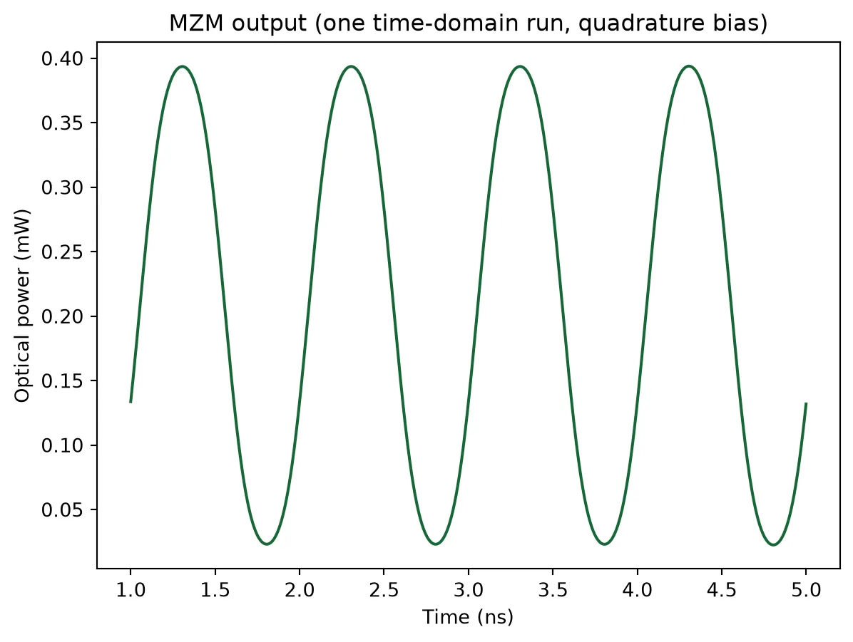
Extinction Ratio: 12.42 dBJunction filter: full RLC implementation (digital IIR)
Section titled “Junction filter: full RLC implementation (digital IIR)”The junction voltage division is modeled by the second-order transfer function:
or equivalently in the Laplace domain:
implemented via PhotonForge’s FilterTimeStepper with family='digital' using discretized IIR coefficients computed at the simulation sampling rate.
Parameters (lumped over the active modulator length)
Section titled “Parameters (lumped over the active modulator length)”- pF
- pH (empirical fit value)
Discretization
Section titled “Discretization”The continuous-time transfer function is converted to discrete-time using the bilinear (Tustin) transform at sampling rate , where is the simulation time step. Because varies across the frequency sweep (), the digital filter coefficients are recomputed at each iteration to remain consistent with the simulation sampling rate.
The bilinear transform is accurate when . With , the oversampling factor is large enough that the discretized response matches the analog essentially exactly across the band of interest (1–40 GHz).
What this filter represents
Section titled “What this filter represents”This RLC filter captures the intrinsic junction voltage division - only a fraction of the line-side voltage drops across the depletion capacitance , with the remainder shared between the series resistance and the parasitic inductance . It is applied in addition to the traveling-wave loaded-line model, which already accounts for microwave loss, velocity mismatch, and impedance mismatch along the transmission line.
Interpretation of the parasitic inductance
Section titled “Interpretation of the parasitic inductance”The 5 pH lumped inductance is a fit parameter that captures unmodeled inductive effects, most likely originating from port parasitics (probe contact, pad transition, residual de-embedding) rather than the per-segment via-stack inductance, which is much smaller and effectively absorbed into the 3D FDTD simulation.
What this filter does not model
Section titled “What this filter does not model”- Frequency dependence of and - both are taken as frequency-independent fitting parameters
- Per-segment variation - the filter is a single lumped equivalent of the per-segment voltage divider, exact for the resistive part since is independent of segment length and fill factor; approximate for the inductive part
- Bias-voltage dependence - , , and are evaluated at a single bias point and re-extracted for other bias conditions
import scipy.signal as signal
def compute_rlc_digital_coeffs(l_parasitic, r_tot, c_tot, time_step):    """Discrete-time IIR coefficients for H(s) = 1 / (1 + s*R*C + s^2*L*C) via Tustin."""    b_continuous = [1.0]    a_continuous = [l_parasitic * c_tot, r_tot * c_tot, 1.0]
    fs = 1.0 / time_step    b_discrete, a_discrete = signal.bilinear(b_continuous, a_continuous, fs)
    return tuple(b_discrete), tuple(a_discrete)
@pf.parametric_componentdef create_single_mod_tb(    signal_freq=1e9,    length=10,    v_pp_drive=2.0,    lpf_b=None,    lpf_a=None,):    """Single-arm testbench: CW Laser -> Modulator and RF Source -> digital-IIR LPF -> Modulator."""
    opt_vir = pf.virtual_port_spec(classification="optical")    elec_vir = pf.virtual_port_spec(classification="electrical")
    laser = pfa.cw_laser(power=1e-3)
    mod_model = pf.AnalyticWaveguideModel(        n_eff=n_eff_opt, length=length, propagation_loss=loss_dB_um, n_group=n_group_opt    )    mod_model.time_stepper = pf.TerminatedModTimeStepper(        v_piL=v_piL_linear,        length=length,        n_eff=n_eff_opt,        n_group=n_group_opt,        n_rf=n_rf_freqs,        propagation_loss=loss_dB_um,        rf_propagation_loss=alpha_db_um_freqs,        z0=z0_freqs,        z_load=z_l,        z_source=z_s,        k2=k2_fit,        k3=k3_fit,    )    mod = mod_model.black_box_component(opt_vir, name="Mod1")    mod.add_port(pf.Port((0.5, 0.5), -90, spec=elec_vir), "E0")
    lpf = pfa.filter(family="digital", b=lpf_b, a=lpf_a)
    amplitude_src = (v_pp_drive / 2) / np.sqrt(z_s)    src = pfa.signal_source(        frequency=signal_freq,        amplitude=amplitude_src,        offset=target_v / np.sqrt(z_s),        waveform="sine",    )
    netlist = {        "name": f"Single_Mod_TB_{signal_freq/1e9:.1f}GHz",        "instances": {            "laser": {"component": laser},            "src": {"component": src},            "lpf": {"component": lpf},            "mod": {"component": mod},        },        "connections": [            (("laser", "P0"), ("mod", "P0")),            (("lpf", "E1"), ("mod", "E0")),            (("src", "E0"), ("lpf", "E0")),        ],        "ports": [("mod", "P1")],        "models": [(pf.CircuitModel(), "Circuit")],    }
    return pf.component_from_netlist(netlist)
Frequency Sweep
Section titled “Frequency Sweep”Evaluate EO bandwidth of the modulator via time-domain simulation.
phase_pp_list = []v_ss = 0.1  # Small signal voltagefor f in freqs_ext:    # 1. Time step    time_step = 1.0 / (1000 * f)    duration = 20.0 / f    num_points = int(round(duration / time_step))
    # 2. Digital filter coefficients for this time step    lpf_b, lpf_a = compute_rlc_digital_coeffs(l_parasitic, r_tot, c_tot, time_step)
    # 3. Testbench for this frequency    mod_tb = create_single_mod_tb(        signal_freq=f,        length=length,        v_pp_drive=v_ss,        lpf_b=lpf_b,        lpf_a=lpf_a,    )
    # 4. Time stepper    freq_span = 200 * f    frequencies = f_c + np.linspace(-freq_span / 2, freq_span / 2, 100)
    ts = mod_tb.setup_time_stepper(        time_step=time_step,        carrier_frequency=f_c,        time_stepper_kwargs={"frequencies": frequencies},    )
    # 5. Run    result_td = ts.step(steps=num_points, time_step=time_step, show_progress=False)
    # 6. Optical field    e_field = result_td["P0@0"]
    # Skip the first half (transient)    e_stable = e_field[num_points // 2 :]
    # 7. Phase    phase = np.unwrap(np.angle(e_stable))    phase_pp = np.max(phase) - np.min(phase)    phase_pp_list.append(phase_pp)
phase_array = np.array(phase_pp_list)s21_0 = np.pi * v_ss * length / (vpiL_fit_cm[arg_v] * 1e4)s21_eo_linear = phase_array / s21_0s21_eo_dB = 20 * np.log10(s21_eo_linear)Retrieve the 3 dB electro-optic bandwidth at the target bias point from the parametric sweep and compare against the frequency-domain analytical model.
plt.figure()plt.plot(    freqs_ext * 1e-9,    20 * np.log10(np.abs(h_total)),    label="Frequency-Domain Sim",)plt.plot(freqs_ext / 1e9, s21_eo_dB, "-", label="Time-Domain Sim")plt.axhline(y=-3, color="r", linestyle="--", alpha=0.8, label="-3 dB Bandwidth")
plt.xlabel("Frequency (GHz)")plt.ylabel("EO S21 (dB)")plt.title("Modulator Frequency Response")plt.grid(True)plt.legend()plt.tight_layout()plt.show()