LiDAR System Budget and Technology

Download notebook (.zip)

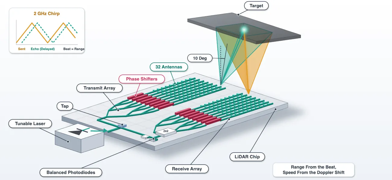
This notebook opens the design of a solid-state LiDAR chip: a frequency-modulated continuous-wave (FMCW) transceiver that steers its beam with an optical phased array (OPA) and measures range and speed by coherent detection. It has no moving parts. The beam is steered in one axis by 32 heaters and in the other by the laser wavelength, and the distance to a target comes out as a beat frequency between the light that went out and the light that came back.

The design is spread over six pages:

System budget and technology (this page): what the LiDAR has to do, what that asks of the chip, and the process stack the chip is built on.
Grating antenna design: the antenna designed step by step, from the pitch and the strip widths to the teeth and the emission angle.
Component library: the splitters, the tap, the thermo-optic phase shifter and the balanced photodiode, each with a model attached.
Chip layout and verification: two phased arrays, the receiver, the heater routing to 64 pads, and the checks that prove the mask is wired as drawn.
Beam steering and thermal budget: the far field of the drawn array, its field of view and sidelobes, and the heater power the steering costs.
FMCW ranging: the assembled chip driven with a chirped laser against moving targets, ending in a range spectrum and a one-axis scene image.

Most of a LiDAR chip is passive silicon. Three questions cannot be answered from the layout alone: whether the drawn aperture collects enough light to range a target at ten metres, how far the beam moves per milliwatt of heater power, and where the antennas point. They need a mode solver, a heat solver and an FDTD solver that read the same technology, which this page sets up. The page starts from the system requirements, because every dimension on the chip follows from one of them.

The LiDAR chip

The transceiver has a transmit array and a receive array, because there is no circulator on a chip and a shared aperture would put the antenna reflections into the receiver far above the return from any target. Light enters from an external tunable laser through an edge coupler. A small tap takes the local oscillator (LO) for the receiver, and the rest goes to the transmit OPA. The receive OPA is an identical copy: light collected by its 32 antennas is combined into one waveguide and mixed with the LO in a 2x2 coupler, and two germanium photodiodes take the difference.

Each OPA is a 1x2 splitter tree to 32 channels, a thermo-optic phase shifter per channel, and 32 grating antennas 1.3 um apart. The heaters set a phase ramp across the array, which steers the beam in the lateral direction, perpendicular to the antennas. The gratings emit at an angle that depends on wavelength, which steers the beam in the longitudinal direction, along the antennas, when the laser is tuned. Together they scan a two-dimensional field of view. The two angles are the lateral angle $\psi$ and the longitudinal angle $\theta$ , both measured from the surface normal (Hulme et al., Opt. Express 23, 5861 (2015)).

Ranging works by chirping the laser frequency linearly over a bandwidth $B$ in a time $T$ . The light returning from a target at range $R$ is delayed by $\tau = 2R/c$ and therefore lags the LO in frequency by

f_b = \frac{B}{T}\,\tau = \frac{2 R B}{c T},

which appears as a beat tone on the balanced photodiodes. A moving target adds a Doppler shift $f_d = 2 v / \lambda$ to that tone. Chirping up and then down gives two beats, $f_b - f_d$ and $f_b + f_d$ , so one triangular chirp yields both range and radial speed. Two targets are resolved when their beats differ by one bin, $1/T$ , which corresponds to a range difference of

\Delta R = \frac{c}{2 B}.

The chirp bandwidth sets the resolution and the chirp time sets the beat frequency per metre. Neither depends on the chip. The chip determines the beam and the fraction of the light that comes back.

import matplotlib.pyplot as plt
import numpy as np
import photonforge as pf
import tidy3d as td

# Keep the solver logs quiet; warnings are still raised as exceptions
td.config.logging.level = "ERROR"

lda0 = 1.55  # Design wavelength, um. Everything in this series references it.
f0 = pf.C_0 / lda0  # Design frequency, Hz
c0 = pf.C_0 * 1e-6  # Speed of light in m/s, for the ranging arithmetic
h_planck = 6.626e-34  # Planck constant, J s, for the photon energy

Ranging budget

The chirp is 2 GHz in 10 us. A 2 GHz sweep is within reach of a current-tuned distributed feedback laser or of an external-cavity laser with a linearization loop. The thermal phase shifters settle in a few tens of microseconds, comparable to the chirp. The numbers below follow from these two values.

b_chirp = 2e9  # Chirp bandwidth (Hz)
t_chirp = 10e-6  # Duration of one chirp ramp (s)
r_design = 10.0  # Range used for the headline numbers (m)
v_design = 10.0  # Radial speed used for the Doppler example (m/s)

# Range resolution set by the chirp bandwidth
dr = c0 / (2 * b_chirp)

# Beat frequency per metre of range, from the chirp slope and the round trip
beat_per_m = 2 * b_chirp / (c0 * t_chirp)

# Doppler shift per metre per second of radial speed
doppler_per_mps = 2 / (lda0 * 1e-6)

print(f"range resolution      {dr * 100:.1f} cm")
print(
    f"beat frequency        {beat_per_m * 1e-6:.2f} MHz per metre, "
    f"{beat_per_m * r_design * 1e-6:.1f} MHz at {r_design:.0f} m"
)
print(
    f"Doppler shift         {doppler_per_mps * 1e-6:.2f} MHz per m/s, "
    f"{doppler_per_mps * v_design * 1e-6:.1f} MHz at {v_design:.0f} m/s"
)
print(
    f"range and speed beats {(beat_per_m * r_design - doppler_per_mps * v_design) * 1e-6:.1f} and "
    f"{(beat_per_m * r_design + doppler_per_mps * v_design) * 1e-6:.1f} MHz on a triangular chirp"
)

range resolution      7.5 cm
beat frequency        1.33 MHz per metre, 13.3 MHz at 10 m
Doppler shift         1.29 MHz per m/s, 12.9 MHz at 10 m/s
range and speed beats 0.4 and 26.2 MHz on a triangular chirp

At ten metres, the Doppler shift of a target moving at car speed equals the range beat. This is why the chirp is triangular rather than a sawtooth. With an up-chirp alone, a receding target at 10 m would read as a stationary one at 20 m.

Beam and aperture budget

The array has $N$ antennas at pitch $d$ . In the lateral direction the beam width is set by the aperture $N d$ and the field of view by the pitch: a phase ramp steers the main lobe until the first grating lobe enters at the opposite edge, which happens at

\psi_\text{FOV} = 2 \arcsin\left(\frac{\lambda}{2 d}\right), \qquad \Delta\psi \approx \frac{\lambda}{N d}.

In the longitudinal direction the beam width is set by the antenna length $L$ , which is how far the grating takes to radiate the light out. The number of resolvable beam positions in each axis is the field of view divided by the beam width.

The pitch is a compromise. At half a wavelength there would be no grating lobes at all, but the antennas would be 0.8 um apart and would couple to each other over a millimetre of length. At two micrometres they are isolated, but the field of view is 45 degrees and the first grating lobe of a broadside beam sits at 51 degrees, where, as the antenna page shows, the antenna still radiates strongly. The pitch here is 1.3 um, below the wavelength, so a broadside beam has no grating lobe in the visible half-space at all and the lobe only enters at the edge of the scan. This is the pitch of the 512-element arrays of Miller et al. [2] and the sub-wavelength arrays of Zhang et al. [3]. The antennas are then 0.8 um apart, and the antenna page keeps them from coupling by alternating two waveguide widths so that neighbours are detuned.

n_ch = 32  # Antennas per array
# Antenna pitch (um), below the wavelength so a broadside beam has no grating lobe
pitch = 1.3
# Antenna length (um), set on the antenna page by the grating strength
l_antenna = 1050.0

# Lateral aperture, across the antennas
aperture_x = n_ch * pitch

# Beam widths in the two axes, from the two aperture dimensions
width_lateral = np.degrees(lda0 / aperture_x)
width_longitudinal = np.degrees(lda0 / l_antenna)

# Lateral field of view, limited by the first grating lobe
fov_x = 2 * np.degrees(np.arcsin(lda0 / (2 * pitch)))

print(f"aperture               {aperture_x:.0f} um x {l_antenna:.0f} um")
print(
    f"beam width             {width_lateral:.2f} deg lateral, {width_longitudinal:.3f} deg longitudinal"
)
print(f"field of view          {fov_x:.1f} deg lateral")
print(f"resolvable positions   {fov_x / width_lateral:.0f} lateral")

aperture               42 um x 1050 um
beam width             2.13 deg lateral, 0.085 deg longitudinal
field of view          73.2 deg lateral
resolvable positions   34 lateral

The number of resolvable lateral beam positions equals the number of antennas. An array of $N$ elements has $N$ degrees of freedom, so it forms $N$ distinct beams inside its grating-lobe-free field of view.

The same aperture sets how much light comes back. A diffuse (Lambertian) target of reflectivity $\rho$ at range $R$ scatters the light it receives into a hemisphere, and the receive aperture $A$ collects the fraction

\frac{P_\text{rx}}{P_\text{tx}} = \rho\,\frac{A}{\pi R^2}.

Coherent detection then compares that return with the local oscillator. With the LO strong enough that its shot noise dominates, the signal-to-noise ratio in one chirp is the number of returned photons collected during the chirp,

\mathrm{SNR} = \frac{\eta\,P_\text{rx}\,T}{h \nu},

with $\eta$ the detector quantum efficiency. It follows from the responsivity $\mathcal{R}$ of the photodiode, $\eta = \mathcal{R}\, h\nu / q$ : the 0.9 A/W of the germanium photodiode on the component page gives 0.72 at 1550 nm. This is the shot-noise limit. The photodiode model on the ranging page generates this shot noise and can add the thermal noise of the amplifier.

p_laser = 10e-3  # Laser power at the fibre (W)
loss_facet = 1.5  # Edge coupler loss (dB)
loss_tap = 0.5  # Loss of the 10 percent local-oscillator tap (dB)
loss_tree = 5 * 0.2  # Five splitter stages at 0.2 dB excess loss each (dB)
# Antenna efficiency measured on the antenna page: light radiated and reaching the air (dB)
loss_antenna = 3.6
rho_dark = 0.1  # Reflectivity of a dark diffuse target
rho_bright = 0.8  # Reflectivity of a white wall
# Photodiode responsivity (A/W), the value the component page builds in
responsivity = 0.9
q_electron = 1.602e-19  # Electron charge (C)
# Quantum efficiency from the responsivity: one electron per photon is q / (h nu) amperes per watt
quantum_efficiency = responsivity * h_planck * f0 / q_electron
snr_min = 10.0  # Detection threshold (dB)

# Power radiated by the transmit array
p_tx = p_laser * 10 ** (-(loss_facet + loss_tap + loss_tree + loss_antenna) / 10)

# Light collected by the receive array loses the same tree and antenna fraction on the way in
loss_rx = loss_antenna + loss_tree

# Receive aperture in square metres
a_rx = aperture_x * 1e-6 * l_antenna * 1e-6

# Photon energy at the design wavelength
e_photon = h_planck * f0

# Returned power and shot-noise-limited SNR against range for both targets
r = np.linspace(1, 50, 500)
snr_db = {}
for name, rho in (("10 % target", rho_dark), ("80 % target", rho_bright)):
    p_rx = p_tx * rho * a_rx / (np.pi * r**2) * 10 ** (-loss_rx / 10)
    snr = quantum_efficiency * p_rx * t_chirp / e_photon
    snr_db[name] = 10 * np.log10(snr)
    # Range at which the SNR crosses the detection threshold
    r_max = np.interp(-snr_min, -snr_db[name], r)
    p_rx_design = np.interp(r_design, r, p_rx)
    print(
        f"{name}: {p_rx_design * 1e15:.0f} fW returned at {r_design:.0f} m, "
        f"SNR {np.interp(r_design, r, snr_db[name]):.0f} dB, "
        f"{snr_min:.0f} dB reached at {r_max:.0f} m"
    )
print(
    f"\nradiated power {10 * np.log10(p_tx * 1e3):.1f} dBm, "
    f"return at {r_design:.0f} m is {10 * np.log10(rho_dark * a_rx / (np.pi * r_design**2)):.0f} dB "
    f"below it for the dark target"
)

fig, ax = plt.subplots(1, 2, figsize=(11, 4))

# Range and Doppler beats against range, for a stationary and an approaching target.
# The photodiode sees the magnitude of the beat, hence the absolute value.
ax[0].plot(r, beat_per_m * r * 1e-6, label="stationary")
ax[0].plot(
    r,
    np.abs(beat_per_m * r - doppler_per_mps * v_design) * 1e-6,
    "--",
    label=f"approaching at {v_design:.0f} m/s, up-chirp",
)
ax[0].plot(
    r,
    (beat_per_m * r + doppler_per_mps * v_design) * 1e-6,
    ":",
    label=f"approaching at {v_design:.0f} m/s, down-chirp",
)
ax[0].set_xlabel("range (m)")
ax[0].set_ylabel("beat frequency (MHz)")
ax[0].set_title("beat frequency")
ax[0].legend()

# Shot-noise-limited SNR against range, with the detection threshold
for name, values in snr_db.items():
    ax[1].plot(r, values, label=name)
ax[1].axhline(snr_min, color="gray", linestyle="--", linewidth=1)
ax[1].set_xlabel("range (m)")
ax[1].set_ylabel("SNR in one chirp (dB)")
ax[1].set_title("coherent SNR, shot-noise limit")
ax[1].set_ylim(-10, 40)
ax[1].legend()
plt.tight_layout()
plt.show()

10 % target: 11 fW returned at 10 m, SNR -2 dB, 10 dB reached at 2 m
80 % target: 84 fW returned at 10 m, SNR 7 dB, 10 dB reached at 7 m

radiated power 3.4 dBm, return at 10 m is -109 dB below it for the dark target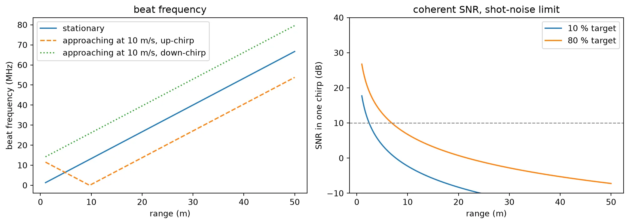

The up-chirp curve for the approaching target folds at ten metres. The range beat grows with distance while the Doppler shift is fixed by the speed, and at that range the two cancel: the light returning from the target has exactly the frequency the local oscillator has now. The photodiode measures a beat frequency without a sign, so on the near side of the fold the tone rises again and a target at 5 m is indistinguishable from one at 15 m. Only the down-chirp, where range and Doppler add, breaks the tie, which is the second reason for the triangular waveform.

The return from a dark target at ten metres is more than a hundred decibels below the radiated power, because the aperture, 42 um by 1 mm, subtends a small solid angle at ten metres. Coherent detection counts photons over the whole chirp, which makes tens of femtowatts detectable. Even so, a dark target is below the threshold at ten metres, and a white wall is detected to seven metres. These numbers include the aperture only. The ranging page rebuilds the budget with every loss the later pages measure, with the true directivity of the beam, and with the polarization and the speckle of a rough target. It arrives at about two metres for the dark target and five for the wall, before a speckle margin. Chip-scale phased arrays in the literature reach a few metres for the same reason. Systems that reach hundreds of metres put a lens in front of the chip or grow the aperture to millimetres. The chip offers two levers: the antenna length, set by how weakly the grating radiates, and the chirp time, which trades measurement rate for photons.

Requirement	Value	What it sets
Range resolution	7.5 cm	chirp bandwidth 2 GHz
Range and speed together	triangular chirp	two beats per measurement
Lateral field of view	73 deg	antenna pitch 1.3 um
Lateral beam width	2.1 deg	32 antennas
Longitudinal beam width	0.085 deg	1050 um antennas
Detection range, 10 dB SNR	2 m dark target, 7 m white wall	the aperture
Second axis	wavelength tuning	grating dispersion, measured below

Process stack

The chip is built on the same platform as the Optical I/O transceiver series: 220 nm silicon-on-insulator with a resistive heater metal, germanium for the detectors and one thick routing metal. One thing differs. The LiDAR has no modulator junctions, so the four implant layers and the charge models are left out; the implants that contact the photodiode belong to the germanium module and are not drawn separately, which is how a foundry delivers the detector as a fixed cell. One thing is added: a partial etch that leaves a 70 nm slab, which every foundry offers for rib waveguides. The antennas use it for their teeth. The coherent LiDAR chip of Poulton et al. [1] corrugated the sidewalls of a strip in the full etch by a few tens of nanometres. A grating weak enough to radiate over a millimetre needs teeth of about 50 nm that way, at the edge of what lithography reproduces. A tooth that is only 70 nm tall perturbs the mode far less for the same width, so the same weak grating is made with teeth of 100 to 200 nm, well inside any design rule. The antenna page measures the radiation strength against the tooth length.

Heights are measured from the bottom of the silicon device layer.

Level	z (um)	Material
Handle wafer	below -2.0	Si
Buried oxide	-2.0 to 0	SiO2
Silicon core	0 to 0.22	Si
Partial-etch slab	0 to 0.07	Si
Germanium	0.22 to 0.72	Ge
TiN heater	1.02 to 1.14	TiN
M1 routing	1.60 to 3.60	Al
Air	above 3.60	air

The table includes the handle wafer and the air above the cladding because both shape the antenna’s radiation. A grating antenna radiates downward as well as upward. The downward half reflects off the silicon under the buried oxide, with the 17 percent reflectivity of an oxide-silicon interface, and comes back through the core, where it interferes with the upward half. Whether the two add or cancel depends on the buried-oxide thickness and on the emission angle. The far field therefore cannot be measured in a slab of oxide alone. The antenna page simulates the whole stack from the wafer to the air. The technology carries the wafer and the oxide as blanket rules, and air is the background that fills everything else, so a simulation that reaches those heights sees the real stack.

Two numbers in this table are design choices rather than platform constants:

The heater sits 0.8 um above the silicon. Closer is more efficient, because less heat spreads sideways before reaching the mode, but the mode starts to see the metal. Sixty-four phase shifters make this the single largest entry in the power budget, so the steering page measures what this separation costs.
The routing metal is 2 um thick, so the long feeds to 64 pads dissipate little compared with the heaters they drive.

References

Poulton, C. V., et al. “Coherent solid-state LIDAR with silicon photonic optical phased arrays.” Optics Letters 2017 42 (20), 4091-4094, doi: 10.1364/OL.42.004091.
Miller, S. A., et al. “Large-scale optical phased array using a low-power multi-pass silicon photonic platform.” Optica 2020 7 (1), 3-6, doi: 10.1364/OPTICA.7.000003.
Zhang, Y., et al. “Sub-wavelength-pitch silicon-photonic optical phased array for large field-of-regard coherent optical beam steering.” Optics Express 2019 27 (3), 1929-1940, doi: 10.1364/OE.27.001929.

Materials

Each material is a dictionary with an "optical" entry and an "electrical" entry. PhotonForge uses the first for mode solving and FDTD, and the second when the layout is extruded for a heat simulation. The electrical entry is a MultiPhysicsMedium carrying thermal conductivity, heat capacity and density, which the heat solver needs for the steady-state phase-shifter efficiency and for its time constant.

Titanium nitride is not in the Tidy3D material library, so the heater uses representative index values for a sputtered film at 1550 nm. Its electrical conductivity, 2.3 S/um, is what sets the heater resistance and therefore the drive voltage for a given power.

# Silicon: dispersive optical model, and the thermal properties the heat solver
# needs. Conductivity in W/(um K), capacity in J/(kg K), density in kg/um^3.
si = {
    "optical": td.material_library["cSi"]["Li1993_293K"],
    "electrical": td.MultiPhysicsMedium(
        optical=td.Medium(permittivity=11.7),
        heat=td.SolidSpec(conductivity=148e-6, capacity=711, density=2.33e-15),
        name="Si",
    ),
}

# Buried oxide and cladding, the medium everything else sits in
sio2 = {
    "optical": td.material_library["SiO2"]["Palik_Lossless"],
    "electrical": td.MultiPhysicsMedium(
        optical=td.Medium(permittivity=3.9),
        heat=td.SolidSpec(conductivity=1.38e-6, capacity=740, density=2.2e-15),
        name="SiO2",
    ),
}

# Heater metal. n and k are representative of a sputtered TiN film at 1550 nm.
tin = {
    "optical": td.medium_from_nk(n=2.6, k=4.2, freq=f0),
    "electrical": td.MultiPhysicsMedium(
        optical=td.PECMedium(),
        heat=td.SolidSpec(conductivity=29e-6, capacity=545, density=5.4e-15),
        charge=td.ChargeConductorMedium(
            conductivity=2.3
        ),  # S/um, sets the heater resistance
        name="TiN",
    ),
}

# Routing metal, which carries every heater net out to its bond pad
al = {
    "optical": td.material_library["Al"]["Rakic1995"],
    "electrical": td.MultiPhysicsMedium(
        optical=td.PECMedium(),
        heat=td.SolidSpec(conductivity=237e-6, capacity=900, density=2.7e-15),
        charge=td.ChargeConductorMedium(conductivity=38),
        name="Al",
    ),
}

# Tungsten plugs connect the heater and the detector contacts up to the routing metal
w = {
    "optical": td.material_library["W"]["RakicLorentzDrude1998"],
    "electrical": td.MultiPhysicsMedium(
        optical=td.PECMedium(),
        heat=td.SolidSpec(conductivity=174e-6, capacity=132, density=19.3e-15),
        charge=td.ChargeConductorMedium(conductivity=18),
        name="W",
    ),
}

# Germanium carries the detectors. Its electrical behaviour is a compact model
# on the ranging page, so only optical and thermal properties are needed here.
ge = {
    "optical": td.material_library["Ge"]["Icenogle1976"],
    "electrical": td.MultiPhysicsMedium(
        optical=td.Medium(permittivity=16.0),
        heat=td.SolidSpec(conductivity=60e-6, capacity=320, density=5.32e-15),
        name="Ge",
    ),
}

# Air fills the passivation opening. A fluid does not conduct heat in the solver,
# which is the right boundary for the top surface of the die.
air = {
    "optical": td.Medium(permittivity=1),
    "electrical": td.MultiPhysicsMedium(
        optical=td.Medium(permittivity=1),
        heat=td.FluidSpec(),
        name="Air",
    ),
}

The technology

A technology in PhotonForge has three parts: the drawing layers, the rules that turn masks into 3D structures, and the waveguide cross-sections used as ports.

Layers are the mask levels a designer draws on. Ten are enough for this chip. The layer numbers match the Optical I/O platform, with the slab and implant numbers left unused, so a cell drawn for one chip extrudes correctly on the other.

Extrusion rules say which mask becomes which material over which range in z. Their order matters, since a later rule overrides an earlier one where they overlap. The silicon takes two rules: whatever is drawn on "Si" is 220 nm of silicon, and whatever is drawn on "Si Partial" but not on "Si" is the 70 nm slab. An antenna is a strip on the first layer with teeth on the second.

Ports define the cross-sections the series solves for, and one is enough: the 500 nm strip carries the splitter tree, the phase shifters, all routing, and the antennas. The antenna teeth raise the average index of the strip by less than one percent, so the strip index sets the emission angle to first order. The grating period is estimated from it at the end of this page and corrected on the antenna page.

Wrapping the definition in parametric_technology makes every stack dimension a keyword argument, so the same code can be re-evaluated at a different silicon thickness or core width when the steering page asks how far the emission angle moves with fabrication.

@pf.parametric_technology
def lidar_soi(
    *,
    core_thickness=0.22,
    ge_thickness=0.5,
    box_thickness=2.0,  # buried oxide between the handle wafer and the core
    slab_thickness=0.07,  # silicon left by the partial etch
    heater_separation=0.8,  # oxide between the silicon top and the heater
    heater_thickness=0.12,
    metal_separation=0.46,  # oxide between the heater top and M1
    metal_thickness=2.0,
    core_width=0.5,
    si=si,
    sio2=sio2,
    tin=tin,
    al=al,
    w=w,
    ge=ge,
    air=air,
):
    layers = {
        "Si": pf.LayerSpec(
            (1, 0), description="Silicon, full etch", color="#1f4e7918", pattern="/"
        ),
        "Si Partial": pf.LayerSpec(
            (2, 0),
            description="Silicon, partial etch to a 70 nm slab",
            color="#4f8fc918",
            pattern="\\",
        ),
        "Ge": pf.LayerSpec(
            (7, 0), description="Germanium detector", color="#7a5c9918", pattern="+"
        ),
        "Contact": pf.LayerSpec(
            (10, 0),
            description="Tungsten plug on silicon",
            color="#88888818",
            pattern="solid",
        ),
        "Ge Contact": pf.LayerSpec(
            (11, 0),
            description="Tungsten plug on germanium",
            color="#66666618",
            pattern="solid",
        ),
        "Heater": pf.LayerSpec(
            (12, 0), description="TiN heater", color="#d4a01718", pattern="-"
        ),
        "Via": pf.LayerSpec(
            (13, 0),
            description="Via from heater to M1",
            color="#aaaaaa18",
            pattern="solid",
        ),
        "M1": pf.LayerSpec(
            (14, 0),
            description="Aluminium routing metal",
            color="#b0b0b018",
            pattern="solid",
        ),
        # Mask only: the cladding ends at the top of M1 here, so the opening has no extrusion rule
        "Pad Open": pf.LayerSpec(
            (15, 0), description="Passivation opening", color="#00000018", pattern=":"
        ),
        # Drawing layers, on no mask: they mark where the design may go and where
        # the saw will cut, and the design rule check reads the first of them.
        "FloorPlan": pf.LayerSpec(
            (99, 0), description="Chip area", color="#2e7d5b10", pattern="hollow"
        ),
        "Dicing": pf.LayerSpec(
            (98, 0), description="Dicing street", color="#c8385a10", pattern="hollow"
        ),
    }

    # z = 0 is the bottom of the silicon device layer.
    z_ge = core_thickness + ge_thickness
    z_heater = core_thickness + heater_separation
    z_metal = z_heater + heater_thickness + metal_separation

    extrusion_specs = [
        # Blanket rules first, no mask: the handle wafer and the oxide. Later rules overwrite
        # earlier ones, so the oxide fills the wafer above the buried-oxide floor and the device
        # layers are cut into the oxide. Each rule has one limit at a finite height.
        pf.ExtrusionSpec(pf.MaskSpec(), si, (-pf.Z_INF, 0)),
        pf.ExtrusionSpec(
            pf.MaskSpec(), sio2, (-box_thickness, z_metal + metal_thickness)
        ),
        # Everything drawn on "Si" is full-thickness silicon; "Si Partial" outside it is slab
        pf.ExtrusionSpec(pf.MaskSpec((1, 0)), si, (0, core_thickness)),
        pf.ExtrusionSpec(
            pf.MaskSpec((2, 0)) - pf.MaskSpec((1, 0)), si, (0, slab_thickness)
        ),
        # Ge is grown on a silicon seed, so the mask is intersected with the
        # silicon: none of it can end up floating in oxide.
        pf.ExtrusionSpec(pf.MaskSpec((7, 0)) * (1, 0), ge, (core_thickness, z_ge)),
        # Plugs run from the surface they land on up to the bottom of M1.
        pf.ExtrusionSpec(pf.MaskSpec((10, 0)), w, (core_thickness, z_metal)),
        pf.ExtrusionSpec(pf.MaskSpec((11, 0)), w, (z_ge, z_metal)),
        pf.ExtrusionSpec(
            pf.MaskSpec((12, 0)), tin, (z_heater, z_heater + heater_thickness)
        ),
        pf.ExtrusionSpec(
            pf.MaskSpec((13, 0)), w, (z_heater + heater_thickness, z_metal)
        ),
        pf.ExtrusionSpec(
            pf.MaskSpec((14, 0)), al, (z_metal, z_metal + metal_thickness)
        ),
    ]

    ports = {
        "TE_1550_500": pf.PortSpec(
            description="Strip waveguide, TE, 500 nm",
            width=3.0,  # simulation window, wide enough for the evanescent tail
            limits=(-1.0, 1.0),
            num_modes=1,
            target_neff=3.5,  # the core index, a search hint for the mode solver
            path_profiles=[(core_width, 0, (1, 0))],
        ),
    }

    return pf.Technology(
        name="LiDAR SOI",
        version="1.0",
        layers=layers,
        extrusion_specs=extrusion_specs,
        ports=ports,
        # Air everywhere that no rule fills: above the cladding and beyond the chip.
        background_medium=air,
    )

tech = lidar_soi()
pf.config.default_technology = tech

The three tables below are the technology as a designer sees it: what can be drawn, what each drawn shape becomes, and which cross-sections carry light.

# List every drawing layer with its number, datatype and description
pf.LayerTable(tech.layers)

Name	Layer	Description	Color	Pattern
Si	(1, 0)	Silicon, full etch	#1f4e7918	/
Si Partial	(2, 0)	Silicon, partial etch to a 70… … nm slab	#4f8fc918	\
Ge	(7, 0)	Germanium detector	#7a5c9918	+
Contact	(10, 0)	Tungsten plug on silicon	#88888818	solid
Ge Contact	(11, 0)	Tungsten plug on germanium	#66666618	solid
Heater	(12, 0)	TiN heater	#d4a01718	-
Via	(13, 0)	Via from heater to M1	#aaaaaa18	solid
M1	(14, 0)	Aluminium routing metal	#b0b0b018	solid
Pad Open	(15, 0)	Passivation opening	#00000018	:
Dicing	(98, 0)	Dicing street	#c8385a10	hollow
FloorPlan	(99, 0)	Chip area	#2e7d5b10	hollow

# List the rule that turns each drawing layer into a solid, with its
# z extent and the medium it is made of
pf.ExtrusionTable(tech.extrusion_specs)

#	Mask	Limits (μm)	Opt. Medium	Elec. Medium
0	()	-inf, 0	cSi_Li1993_293K	MultiPhysicsMedium(name='Si',… … optical={'permittivity': 11.7}, heat={'capacity': 711.0, 'conductivity': 0.000148, 'density': 2.33e-15})
1	()	-2, 3.6	SiO2_Palik_LowLoss	MultiPhysicsMedium(name='SiO2',… … optical={'permittivity': 3.9}, heat={'capacity': 740.0, 'conductivity': 1.38e-06, 'density': 2.2e-15})
2	(1, 0)	0, 0.22	cSi_Li1993_293K	MultiPhysicsMedium(name='Si',… … optical={'permittivity': 11.7}, heat={'capacity': 711.0, 'conductivity': 0.000148, 'density': 2.33e-15})
3	(2, 0) - (1, 0)	0, 0.07	cSi_Li1993_293K	MultiPhysicsMedium(name='Si',… … optical={'permittivity': 11.7}, heat={'capacity': 711.0, 'conductivity': 0.000148, 'density': 2.33e-15})
4	(7, 0) * (1, 0)	0.22, 0.72	Ge_Icenogle1976	MultiPhysicsMedium(name='Ge',… … optical={'permittivity': 16.0}, heat={'capacity': 320.0, 'conductivity': 6e-05, 'density': 5.32e-15})
5	(10, 0)	0.22, 1.6	W_RakicLorentzDrude1998	MultiPhysicsMedium(name='W',… … optical={}, heat={'capacity': 132.0, 'conductivity': 0.000174, 'density': 1.93e-14}, charge={'conductivity': 18.0})
6	(11, 0)	0.72, 1.6	W_RakicLorentzDrude1998	MultiPhysicsMedium(name='W',… … optical={}, heat={'capacity': 132.0, 'conductivity': 0.000174, 'density': 1.93e-14}, charge={'conductivity': 18.0})
7	(12, 0)	1.02, 1.14	Lorentz(coeffs=… …((21.840000000000003, 162323815372577.7, 52562735135327.414),))	MultiPhysicsMedium(name='TiN',… … optical={}, heat={'capacity': 545.0, 'conductivity': 2.9e-05, 'density': 5.4e-15}, charge={'conductivity': 2.3})
8	(13, 0)	1.14, 1.6	W_RakicLorentzDrude1998	MultiPhysicsMedium(name='W',… … optical={}, heat={'capacity': 132.0, 'conductivity': 0.000174, 'density': 1.93e-14}, charge={'conductivity': 18.0})
9	(14, 0)	1.6, 3.6	Al_Rakic1995	MultiPhysicsMedium(name='Al',… … optical={}, heat={'capacity': 900.0, 'conductivity': 0.000237, 'density': 2.7e-15}, charge={'conductivity': 38.0})

# List the waveguide cross-sections available as ports, with their widths,
# layer stacks and the number of modes each carries
pf.PortSpecTable(tech.ports)

Name	Classification	Description	Width (μm)	Limits (μm)	Radius (μm)	Modes	Target n_eff	Path profiles (μm)
TE_1550_500	optical	Strip waveguide, TE, 500 nm	3	-1, 1	0	1	3.5	(1, 0): 0.5

Cross-section check

Drawing the cross-sections is the direct check of the extrusion rules. The test cell below holds two devices. The phase shifter is a strip waveguide with a TiN strip above it. The TiN strip ends in two landing areas where vias rise to the M1 feeds; the feeds drive the heater and also drain part of its heat. The antenna is a short piece of grating: the strip with partial-etch teeth on both sides. The phase shifter runs along $y$ , so a cut through $y = 0$ shows its waveguide profile and a cut through $x = 0$ runs along the heater and shows how the feeds reach it. The antenna runs along $x$ . It is shown in plan view at the slab height, where both etches leave silicon, and in a cut across one tooth, which shows the 70 nm shoulder that the partial etch leaves beside the full-height strip. The two phase-shifter cuts run from the handle wafer to the air, so the wafer rule appears as the floor of the stack and the air background as its ceiling.

# Grating period for the test cell (um); the real value is solved below
grating_period = 0.74
corrugation = 0.15  # Width of each partial-etch sidewall tooth (um)
heater_length = 4.0  # Heater length in the test cell (um), a real one is a few hundred
heater_width = 1.0  # Heater width (um)
via_length = 0.5  # Length of the via landing at each heater end (um)

# Build a test cell whose only job is to check the extrusion rules. The shapes
# are plain rectangles, not devices: each one exercises one drawing layer.
xs = pf.Component("cross_section", technology=tech)

# Phase shifter: strip core along y with the heater strip centred above it
y_end = heater_length / 2
xs.add(
    "Si",
    pf.Rectangle((-0.25, -y_end - 1), (0.25, y_end + 1)),
    "Heater",
    pf.Rectangle((-heater_width / 2, -y_end), (heater_width / 2, y_end)),
)

# Vias on the two heater ends, and an M1 feed covering each via and running outward
for sign in (-1, 1):
    y_inner = sign * (y_end - via_length)  # via edge nearest the heater centre
    y_outer = sign * (y_end + 1)  # where the feed leaves the test cell
    xs.add(
        "Via",
        pf.Rectangle((-0.4, y_inner), (0.4, sign * y_end)),
        "M1",
        pf.Rectangle((-heater_width / 2, y_inner), (heater_width / 2, y_outer)),
    )

# Antenna: the strip along x, with a partial-etch tooth on both sidewalls over half of every period
xs.add("Si", pf.Rectangle((6, -0.25), (6 + 5 * grating_period, 0.25)))
for i in range(5):
    x_tooth = 6 + i * grating_period
    xs.add(
        "Si Partial",
        pf.Rectangle(
            (x_tooth, -0.25 - corrugation),
            (x_tooth + grating_period / 2, 0.25 + corrugation),
        ),
    )

# Draw the stack the extrusion rules produced, in four cuts
fig, ax = plt.subplots(
    1, 4, figsize=(18, 3.6), gridspec_kw={"width_ratios": [1, 1.4, 1.6, 1]}
)

# Across the phase shifter: the core with the heater above it, no metal nearby
pf.tidy3d_plot(xs, y=0, ax=ax[0], plot_type="structures", frequency=f0)
ax[0].set_xlim(-2.0, 2.0)
ax[0].set_ylim(-2.6, 4.4)
ax[0].set_title("phase shifter, across the waveguide")

# Along the phase shifter: the heater strip, the vias on its ends and the M1 feeds
pf.tidy3d_plot(xs, x=0, ax=ax[1], plot_type="structures", frequency=f0)
ax[1].set_xlim(-y_end - 1.2, y_end + 1.2)
ax[1].set_ylim(-2.6, 4.4)
ax[1].set_title("phase shifter, along the waveguide")

# The antenna in plan view, at the slab height where both etches show: the toothed outline
pf.tidy3d_plot(xs, z=0.035, ax=ax[2], plot_type="structures", frequency=f0)
ax[2].set_xlim(5.8, 6.2 + 5 * grating_period)
ax[2].set_ylim(-0.6, 0.6)
ax[2].set_title("grating antenna, plan view at slab height")

# Across the antenna through a tooth: the full-height strip with a slab shoulder on each side
pf.tidy3d_plot(
    xs, x=6 + grating_period / 4, ax=ax[3], plot_type="structures", frequency=f0
)
ax[3].set_xlim(-0.8, 0.8)
ax[3].set_ylim(-0.3, 0.5)
ax[3].set_title("antenna, across a tooth")
plt.tight_layout()
plt.show()

Waveguide indices and the emission angle

With the stack defined, the strip can be solved for its mode. Two numbers come out of this that the rest of the series depends on.

The first is the group index of the strip waveguide, which decides how the two phased arrays have to be routed. A path difference $\Delta L$ between two channels adds a phase $2 \pi n_\text{eff} \Delta L / \lambda$ between them, which the heaters can cancel at one wavelength. When the laser is tuned by $\Delta\lambda$ to steer the second axis, that phase moves by

\Delta\phi = \frac{2 \pi n_g \Delta L}{\lambda^2}\,\Delta\lambda,

If it moves by more than a fraction of a radian, the beam is lost at the new wavelength until every heater is reset. The layout page records the length of every channel for this reason, and the steering page turns those lengths into the heater settings each wavelength needs.

The second is the emission angle of the grating. A grating of period $\Lambda$ on a waveguide of effective index $n_\text{eff}$ sends its first diffraction order out of the chip at

\sin\theta = n_\text{eff} - \frac{\lambda}{\Lambda}.

The angle is measured from the surface normal in air, since the oxide above the grating refracts the light back to this angle. The teeth change the index of the grating by less than one percent, so the strip index is enough to estimate the period here; the antenna page measures the correction. A grating that emits exactly vertically reflects strongly back into the waveguide, so gratings point a little off normal, usually by 5 to 15 degrees. This one points 10 degrees off.

The angle also depends on the stack. The light the antenna sends downward reflects off the handle wafer and interferes with the light sent upward. The buried-oxide thickness and the radiation profile of the grating decide where that interference is bright. The antenna page works this out. A grating that radiates equally up and down would find a 2 um oxide dark near the normal and bright on a cone near 35 degrees. The partial-etch grating chosen there radiates asymmetrically and is bright near the normal. Measured on an equal footing, its patterns at 10 and at 20 degrees agree to a quarter of a decibel. Ten degrees is kept, the smallest customary tilt, so the module looks close to the chip normal.

Tuning the laser moves the angle at a rate set by the grating dispersion and the waveguide dispersion together. That rate is the steering slope of the second axis. The waveguide dispersion enters through the group index, since to first order $n_\text{eff}(\lambda) = n_\text{eff} - (n_g - n_\text{eff})\,(\lambda - \lambda_0)/\lambda_0$ .

# One wavelength grid for every mode solve, so the solver cache is reused
wavelengths = np.linspace(1.53, 1.57, 5)
freqs = pf.C_0 / wavelengths

# Solve the strip mode with its group index, at the design wavelength only
strip = pf.port_modes(
    "TE_1550_500", [f0], group_index=True, show_progress=False, verbose=False
)
n_eff_strip = float(np.real(strip.data.n_eff.values.ravel()[0]))
n_group_strip = float(np.real(strip.data.n_group.values.ravel()[0]))
print(f"strip   n_eff = {n_eff_strip:.4f}   n_group = {n_group_strip:.4f}")

# Strip index across the tuning range, to first order from the group index
n_eff_lda = n_eff_strip - (n_group_strip - n_eff_strip) * (wavelengths - lda0) / lda0

# Grating period that emits theta0 from the normal at the design wavelength
# Emission angle at 1550 nm (deg): off normal against back-reflection, small so the module looks near normal
theta0 = 10.0
grating_period = lda0 / (n_eff_strip - np.sin(np.radians(theta0)))

# Emission angle across the tuning range, and its slope
theta = np.degrees(np.arcsin(n_eff_lda - wavelengths / grating_period))
slope = np.polyfit(wavelengths * 1e3, theta, 1)[0]
print(f"\ngrating period {grating_period * 1e3:.0f} nm for {theta0:.0f} deg emission")
print(
    f"wavelength steering {slope:.3f} deg/nm, {slope * (wavelengths[-1] - wavelengths[0]) * 1e3:.1f} deg "
    f"over {(wavelengths[-1] - wavelengths[0]) * 1e3:.0f} nm, "
    f"{abs(slope * (wavelengths[-1] - wavelengths[0]) * 1e3) / width_longitudinal:.0f} beam widths"
)

# Phase drift across the tune for a 100 um path mismatch between two channels
delta_l = 100.0  # Path-length mismatch (um)
delta_phi = (
    2 * np.pi * n_group_strip * delta_l * (wavelengths[-1] - wavelengths[0]) / lda0**2
)
print(
    f"\n{delta_l:.0f} um path mismatch drifts by {delta_phi:.0f} rad over the tune, "
    f"{delta_phi / (2 * np.pi):.1f} waves"
)

fig, ax = plt.subplots(1, 1, figsize=(5.5, 4))
ax.plot(wavelengths * 1e3, theta)
ax.set_xlabel("wavelength (nm)")
ax.set_ylabel("emission angle from normal (deg)")
ax.set_title("wavelength steering")
plt.show()

strip   n_eff = 2.4391   n_group = 4.1782

grating period 684 nm for 10 deg emission
wavelength steering -0.150 deg/nm, -6.0 deg over 40 nm, 71 beam widths

100 um path mismatch drifts by 44 rad over the tune, 7.0 waves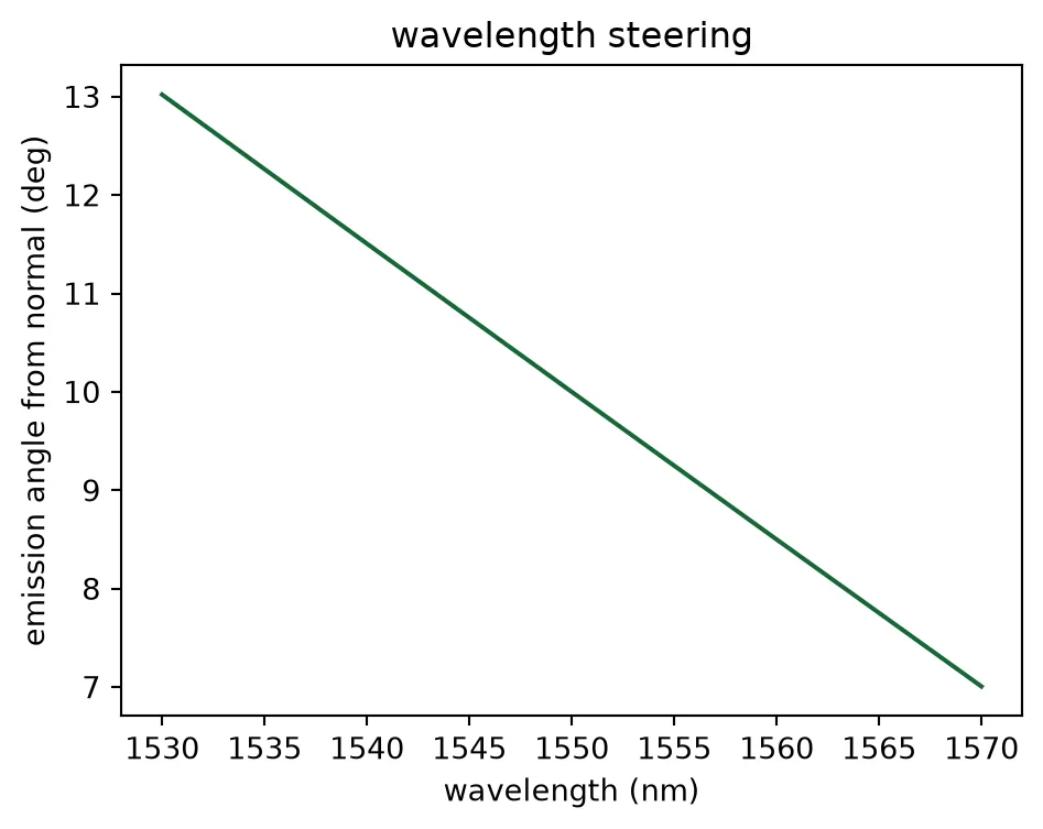

The steering slope is a fraction of a degree per nanometre, so the 40 nm tuning range of the laser scans a few degrees in the longitudinal direction. This is a much smaller field of view than the 73 degrees the phase ramp covers laterally. The beam is also much narrower in that axis, so the number of resolvable positions is comparable. A wider tuning range or a more dispersive grating would widen it, at the cost of laser or antenna efficiency.

The path mismatch shapes the layout. Tens of radians of drift over the tune means that channels of unequal length need their 32 heaters reset at every wavelength step. The layout therefore either equalizes the lengths or records them exactly. Equalizing them is not possible in the space that a 25 um phase-shifter pitch leaves, so the layout page records every channel’s length and the heaters follow a table.

The same layout, for heat

Everything so far used the optical half of each material. Passing classification="electrical" to Component.extrude extrudes the identical layout with the multiphysics half instead. Each solid it returns carries its own medium and converts with to_tidy3d into a structure that a HeatChargeSimulation accepts directly. The phase shifter is drawn once, and its temperature rise per milliwatt and its time constant on the steering page come from that one drawing.

# Extrude the same test cell again, this time selecting the multiphysics media rather
# than the optical ones
structures = [x.to_tidy3d() for x in xs.extrude(classification="electrical")]
print(f"{len(structures)} structures:", sorted({s.medium.name for s in structures}))

# A Scene is enough to render material properties; no solver setup needed yet.
scene = td.Scene(structures=structures, medium=sio2["electrical"])

# Thermal conductivity along the phase shifter, which the heater solve needs
fig, ax = plt.subplots(1, 1, figsize=(7, 4))
scene.plot_structures_heat_charge_property(
    x=0,
    ax=ax,
    property="heat_conductivity",
    hlim=(-y_end - 1.2, y_end + 1.2),
    vlim=(-2.6, 4.4),
)
plt.show()

10 structures: ['Al', 'Si', 'SiO2', 'TiN', 'W']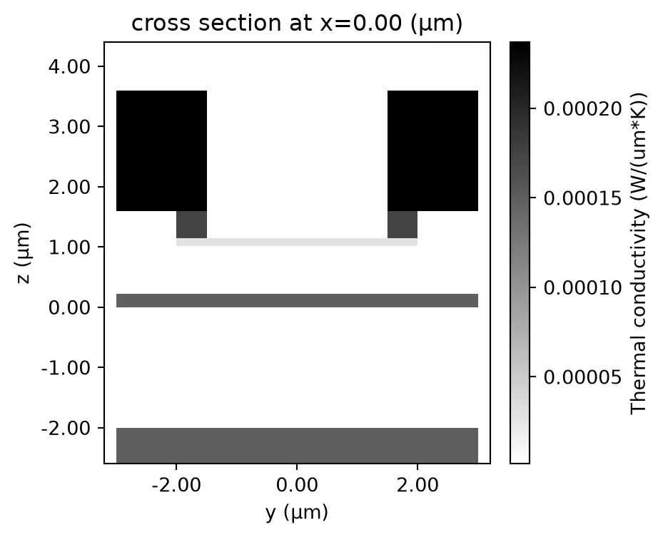

The panel shows the phase shifter as the heat solver sees it, along the waveguide. The TiN strip is the source. The oxide around it conducts a hundred times worse than the metals, so the heat has two ways out: down through the oxide to the silicon core and the substrate, which is the useful path, and out through the tungsten vias into the aluminium feeds, which is lost. The feeds are drawn at the ends of the heater rather than beside it for that reason. The steering page measures how much of the power still leaves that way.

What comes next

The technology is complete. The antenna page designs the grating antenna step by step: the pitch, the strip widths, the radiation strength, the emission angle, and the coupling between antennas 0.8 um apart. The component library then builds the splitters, the tap, the phase shifter and the detector, and attaches a model to each. The chip-level pages steer and range with those models.