800G Coherent Link Budget and Technology

Download notebook (.zip)

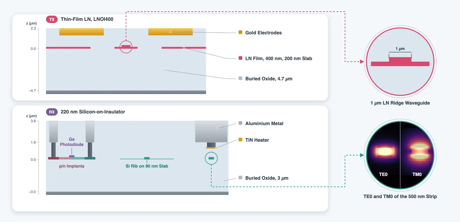
This series designs an 800 Gb/s coherent optical link: a transmitter chip and a receiver chip that carry dual-polarization 16-level quadrature amplitude modulation (DP-16QAM) at 120 GBd over 80 km of fiber. The transmitter is a thin-film lithium niobate (TFLN) chip on the open Luxtelligence LNOI400 process. The receiver is a silicon chip on a 220 nm silicon-on-insulator (SOI) process that this page writes. The series ends with a constellation and a bit error rate (BER) against the optical signal-to-noise ratio (OSNR) of the link.

The design is spread over five pages:

Link budget and technology (this page): what an 800G coherent link asks of the two chips, and the process stacks they are built on.
Transmitter components: the travelling-wave modulator, the multimode interference (MMI) splitter, the bias heater, the polarization rotator-combiner and the edge coupler, on LNOI400.
Receiver components: the edge coupler, the polarization splitter-rotator, the 90 degree hybrid and the germanium photodiode with its amplifier, on the SOI process.
Chip layout and verification: both chips drawn, with design rule checks and a layout-versus-schematic check on each.
Link simulation: both chips, the fiber, the amplifier and the receiver signal processing in one time-domain simulation, ending in BER against OSNR.

References

Kikuchi, Kazuro. “Fundamentals of coherent optical fiber communications.” Journal of Lightwave Technology 2016 34 (1), 157-179, doi: 10.1109/JLT.2015.2463719.
Xu, Mengyue, et al. “Dual-polarization thin-film lithium niobate in-phase quadrature modulators for terabit-per-second transmission.” Optica 2022 9 (1), 61-62, doi: 10.1364/OPTICA.449691.
Luxtelligence LNOI400 process design kit and design manual, available from luxtelligence.ai/resources.
Cheben, Pavel, et al. “Broadband polarization independent nanophotonic coupler for silicon waveguides with ultra-high efficiency.” Optics Express 2015 23 (17), 22553-22563, doi: 10.1364/OE.23.022553.
Chen, Hongtao, et al. “-1 V bias 67 GHz bandwidth Si-contacted germanium waveguide p-i-n photodetector for optical links at 56 Gbps and beyond.” Optics Express 2016 24 (5), 4622-4631, doi: 10.1364/OE.24.004622.

The coherent link

A coherent link sends information in the amplitude and the phase of the optical field, on both polarizations, and recovers the field at the receiver by mixing it with a local oscillator (LO) laser. 16QAM puts 4 bits on each symbol of each polarization, so at a symbol rate $R_s$ the line rate is $8 R_s$ .

The two chips do separate jobs, which is also how coherent optics is built commercially: the transmitter needs the Pockels effect, which lithium niobate has and silicon does not, and the receiver needs a photodetector, which germanium on silicon provides and thin-film lithium niobate does not.

Transmitter (LNOI400). An edge coupler takes the laser light onto the chip and a 1x2 MMI splits it between two IQ modulators, one per polarization. Each IQ modulator is a pair of travelling-wave Mach-Zehnder modulators (MZMs) biased at their null, one for the in-phase (I) and one for the quadrature (Q) part of the field, combined with a 90 degree phase offset set by a heater. A polarization rotator-combiner (PRC) turns one of the two outputs into the transverse-magnetic (TM) mode, combines both into one waveguide, and an edge coupler sends them into the fiber. Xu et al. [2] demonstrated this architecture on TFLN.
Receiver (SOI). An edge coupler takes both polarizations from the fiber. A polarization splitter-rotator (PSR) separates them and rotates the TM part into the transverse-electric (TE) mode, so the rest of the chip handles TE only. Each polarization then meets half of the LO in a 90 degree hybrid, whose four outputs feed two balanced pairs of germanium photodiodes. Each pair drives a transimpedance amplifier (TIA). The four output voltages are the I and Q parts of the two polarizations.

Digital signal processing after the receiver undoes what the fiber did: chromatic dispersion, the random rotation of the polarization, the frequency offset between the two lasers and their phase noise.

import luxtelligence_lnoi400_forge as lx
import matplotlib.pyplot as plt
import numpy as np
import photonforge as pf
import tidy3d as td
from scipy.optimize import brentq
from scipy.special import erfc

# Keep the solver logs quiet; warnings are still raised as exceptions
td.config.logging.level = "ERROR"

lda0 = 1.55  # Design wavelength (um). Everything in this series references it.
f0 = pf.C_0 / lda0  # Design frequency (Hz); pf.C_0 is the speed of light in um/s
q_electron = 1.602e-19  # Electron charge (C), for the photocurrent noise

14:33:48 -03 WARNING: The material-library variant 'Palik_Lossless' is          
             deprecated and maps to 'Palik_LowLoss' because it contains a tiny  
             fitted loss despite its name. Use 'Palik_NoLoss' where available   
             for a zero-loss Palik model.

Symbol rate and the required OSNR

The forward error correction (FEC) of an 800G coherent link corrects a pre-FEC BER of about 2 × 10⁻² down to an error-free output, at about 15 % overhead. 800 Gb/s of payload therefore needs about 960 Gb/s on the line, which DP-16QAM carries at 120 GBd.

The noise that sets the BER of an amplified link is the amplified spontaneous emission (ASE) of the optical amplifiers. ASE is broadband: it spans the whole gain band of the amplifier, tens of nanometres, and is flat across the 1 nm or so that a 120 GBd signal occupies. Its level is therefore given as a power per bandwidth, and the OSNR is the signal power over the ASE power of both polarizations counted in a fixed slice of spectrum, the reference bandwidth. The convention is 0.1 nm, the resolution bandwidth of the optical spectrum analyzers used to measure it, which is $B_\text{ref} = c\,\Delta\lambda / \lambda^2 = 12.5$ GHz at 1550 nm. It is a unit of measurement, not a property of the amplifier or of the signal, so OSNR values compare across links of any symbol rate. The noise the receiver actually sees is the ASE inside the signal’s own bandwidth. With matched filtering, the signal-to-noise ratio per symbol on each polarization is

\mathrm{SNR} = \frac{E_s}{N_0} = \mathrm{OSNR}\,\frac{B_\text{ref}}{R_s},

since each polarization carries half the signal and sees half the ASE. For Gray-coded 16QAM in additive white Gaussian noise the BER follows from the error probability of each of the two 4-level axes [1]:

\mathrm{BER} \approx \frac{3}{8}\,\mathrm{erfc}\sqrt{\frac{\mathrm{SNR}}{10}}.

This curve is the reference the link page compares the simulated link against.

baud = 120e9  # Symbol rate (Bd)
bits_per_symbol = 4  # 16QAM
b_ref = 12.5e9  # OSNR reference bandwidth, 0.1 nm at 1550 nm (Hz)
ber_fec = 2e-2  # Pre-FEC BER the error correction can repair

# Line rate: two polarizations, four bits per symbol each
line_rate = 2 * bits_per_symbol * baud
print(f"line rate {line_rate * 1e-9:.0f} Gb/s at {baud * 1e-9:.0f} GBd")

# Gray-coded 16QAM in white Gaussian noise, SNR = Es/N0 per polarization
def ber_16qam(snr):
    return 3 / 8 * erfc(np.sqrt(snr / 10))

# OSNR in dB from the SNR per symbol, and back
osnr_db = np.linspace(14, 32, 200)
snr = 10 ** (osnr_db / 10) * b_ref / baud
ber = ber_16qam(snr)

# Required OSNR at the FEC threshold and at a tighter BER for comparison
for target in (ber_fec, 1e-3):
    snr_req = brentq(lambda s: ber_16qam(s) - target, 1, 1e4)
    osnr_req = 10 * np.log10(snr_req * baud / b_ref)
    print(
        f"BER {target:.0e}: SNR {10 * np.log10(snr_req):.1f} dB, required OSNR {osnr_req:.1f} dB"
    )

fig, ax = plt.subplots(1, 1, figsize=(5.5, 4))
ax.semilogy(osnr_db, ber)
ax.axhline(ber_fec, color="0.5", ls="--", lw=1)
ax.set_xlabel("OSNR in 0.1 nm (dB)")
ax.set_ylabel("BER")
ax.set_ylim(1e-6, 0.3)
ax.set_title("DP-16QAM at 120 GBd")
plt.show()

line rate 960 Gb/s at 120 GBd
BER 2e-02: SNR 12.7 dB, required OSNR 22.5 dB
BER 1e-03: SNR 16.5 dB, required OSNR 26.4 dB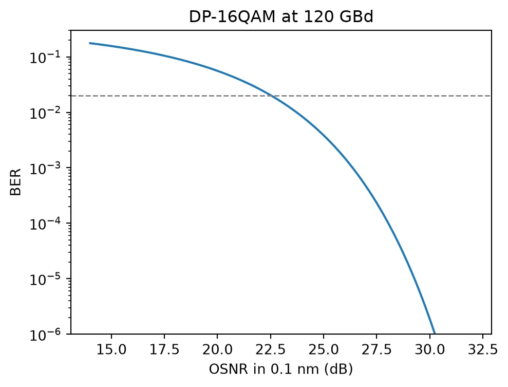

At the FEC threshold the link needs an OSNR of about 22.5 dB. This is the number the whole chip budget is measured against: every impairment the chips add, such as a limited bandwidth, an unbalanced hybrid or a skew between I and Q, shows up as extra OSNR needed for the same BER.

The bandwidth the chips need follows from the pulse shape. The transmitter shapes each symbol with a root-raised-cosine filter of roll-off 0.1, so the signal occupies $\pm (1 + 0.1) R_s / 2 = \pm 66$ GHz around the carrier. The modulator, the photodiode and the amplifier do not have to pass all of it: equalization in the signal processing recovers a response that falls off smoothly, and electro-optic 3 dB bandwidths of about half the symbol rate are common in 120 GBd systems. The two component pages measure these bandwidths, and the link page measures what they cost in OSNR.

Receiver noise budget

Beyond the ASE, the receiver adds noise of its own: the shot noise of the photocurrent and the input noise of the TIA. A strong LO raises the signal above both, because the balanced photocurrent of one quadrature is the beat between the signal field and the LO field,

i_I(t) = \mathcal{R}\,\sqrt{P_s P_\text{LO}}\,\cos\varphi(t),

with $\mathcal{R}$ the responsivity, $P_s$ and $P_\text{LO}$ the signal and LO power entering the hybrid and $\varphi$ the phase between them. Summed over I and Q its mean square power is $\mathcal{R}^2 P_s P_\text{LO}$ . Each of the four photodiodes of a hybrid receives a quarter of the LO, whose shot noise has a spectral density $2 q \mathcal{R} P_\text{LO}/4$ , and each TIA adds its input noise density $i_n^2$ . A balanced pair has two of each. A matched filter passes noise in a bandwidth $R_s / 2$ on each of the two quadratures, so the SNR set by the receiver alone is

\mathrm{SNR}_\text{rx} = \frac{\mathcal{R}^2 P_s P_\text{LO}} {2 \cdot 2\left(i_n^2 + 2 q \mathcal{R} P_\text{LO}/4\right) R_s / 2}.

The cell below evaluates it for the input powers of the link page: −5 dBm of signal in both polarizations at the receiver fiber and a 0 dBm LO. The losses are the receiver component values measured on the receiver page. The photodiode responsivity is that of the photodiode of Chen et al. [5], and the TIA noise that of the amplifier the receiver page models.

p_signal_dbm = -5.0  # Signal at the receiver fiber, both polarizations (dBm)
p_lo_dbm = 0.0  # Local oscillator at its fiber (dBm)
loss_ec = 0.4  # Edge coupler loss (dB)
loss_psr = 0.5  # Polarization splitter-rotator loss (dB)
responsivity = 0.74  # Photodiode responsivity (A/W)
i_noise = 12.2e-12  # TIA input noise current density (A/rtHz)

# Signal per polarization and LO per hybrid, as they enter the hybrids. The PSR
# separates the polarizations and a 1x2 splitter shares the LO between the two hybrids.
p_s = 1e-3 * 10 ** ((p_signal_dbm - 3 - loss_ec - loss_psr) / 10)
p_lo = 1e-3 * 10 ** ((p_lo_dbm - 3 - loss_ec) / 10)

# Beat signal power of one polarization, I and Q together (A^2)
signal = responsivity**2 * p_s * p_lo

# Noise densities of one balanced pair: two TIA inputs and two LO shot-noise terms (A^2/Hz)
tia = 2 * i_noise**2
shot = 2 * (2 * q_electron * responsivity * p_lo / 4)

# Two quadratures, each in a matched-filter noise bandwidth of half the symbol rate
noise = 2 * (tia + shot) * baud / 2
snr_rx = signal / noise
print(f"photocurrent per photodiode from the LO {responsivity * p_lo / 4 * 1e6:.0f} uA")
print(
    f"noise density per pair: TIA {np.sqrt(tia) * 1e12:.1f} pA/rtHz, "
    f"LO shot noise {np.sqrt(shot) * 1e12:.1f} pA/rtHz"
)
print(f"receiver-limited SNR {10 * np.log10(snr_rx):.1f} dB")

# The same SNR expressed as the OSNR that would give it, for comparison with the threshold
print(
    f"equivalent OSNR of the receiver noise {10 * np.log10(snr_rx * baud / b_ref):.1f} dB"
)

# Independent noises add, 1/SNR = 1/SNR_ase + 1/SNR_rx, so the ASE may use what the receiver leaves
snr_fec = brentq(lambda s: ber_16qam(s) - ber_fec, 1, 1e4)
snr_ase = 1 / (1 / snr_fec - 1 / snr_rx)
osnr_fec = 10 * np.log10(snr_fec * baud / b_ref)
osnr_with_rx = 10 * np.log10(snr_ase * baud / b_ref)
print(f"required OSNR at the FEC threshold, noiseless receiver: {osnr_fec:.2f} dB")
print(f"required OSNR at the FEC threshold, this receiver: {osnr_with_rx:.2f} dB")

photocurrent per photodiode from the LO 85 uA
noise density per pair: TIA 17.3 pA/rtHz, LO shot noise 7.4 pA/rtHz
receiver-limited SNR 28.8 dB
equivalent OSNR of the receiver noise 38.7 dB
required OSNR at the FEC threshold, noiseless receiver: 22.53 dB
required OSNR at the FEC threshold, this receiver: 22.64 dB

The 38.7 dB is not a requirement on the link. It measures how noisy the receiver is, in the units of the link: the receiver adds as much noise as an optical link with an OSNR of 38.7 dB would. The ASE and the receiver noise are independent, so their powers add,

\frac{1}{\mathrm{SNR}} = \frac{1}{\mathrm{SNR}_\text{ASE}} + \frac{1}{\mathrm{SNR}_\text{rx}},

and the total must still reach the 12.7 dB the FEC threshold needs. The receiver’s share is 16 dB below that, so the ASE can take almost the whole noise budget: the OSNR the link must deliver rises from 22.53 to 22.64 dB, a penalty of about 0.1 dB. A receiver whose own noise were equivalent to 22.5 dB would leave nothing for the ASE, and no OSNR would be enough. The link is therefore limited by the ASE, as an amplified 80 km link should be. The TIA noise is larger than the LO shot noise at this LO power. A stronger LO would raise the signal further, but the photodiodes saturate near 1 mA of photocurrent, and the link page keeps the LO at 0 dBm.

Requirement	Value	What it sets
Line rate	960 Gb/s	DP-16QAM at 120 GBd
Required OSNR, BER 2 × 10⁻²	22.5 dB	the reference for every penalty
Signal bandwidth	±66 GHz	root-raised-cosine, roll-off 0.1
Receiver noise	0.1 dB OSNR penalty	LO 0 dBm, signal −5 dBm

Transmitter technology: LNOI400

The transmitter uses the LNOI400 process of Luxtelligence [3]: a 400 nm film of x-cut lithium niobate on 4.7 um of buried oxide, etched halfway to leave a 200 nm slab, with gold transmission lines for the travelling-wave electrodes and a metal heater layer. The process design kit (PDK) is available as the luxtelligence_lnoi400_forge package, which provides the technology and the cell library. The design manual and the rule deck used on the layout page are available from the Luxtelligence website.

# Load the PDK technology; every transmitter component and the transmitter die use it
tech_tx = lx.lnoi400()
tech_tx.layers

Name	Layer	Description	Color	Pattern
LN_RIDGE	(2, 0)	LN etch (ridge)	#7d57de18	/
LT_RIDGE_PERIODIC	(2, 1)	LN etch (ridge, periodic… … features)	#ff00ff18	\\
LN_SLAB	(3, 0)	LN etch (full)	#00008018	//
SLAB_NEGATIVE	(3, 1)	Slab etch negative	#6750bf18	/
LABELS	(4, 0)	Labels (LN etch)	#5179b518	\|
CHIP_CONTOUR	(6, 0)	Usable floorplan area	#ffc6b818	-
CHIP_EXCLUSION_ZONE	(6, 1)	Final chip boundaries	#00fe9c18	\|\|
TL	(21, 0)	Metal transmission lines	#3503fc18	=
HT	(21, 1)	Metal heaters	#3503fc18	.
ALIGN	(31, 0)	Alignment markers (LN etch)	#d4467c18	:
ERROR	(50, 1)	Error markers	#c7031c18	xx
DOC	(201, 0)	Labels for GDS layout (not… … fabricated)	#857b7518	++
WAFER	(990, 0)	Wafer	#47332818	hollow

# The waveguide cross-sections the PDK defines as ports
tech_tx.ports

Name	Classification	Description	Width (μm)	Limits (μm)	Modes	Target n_eff	Path profiles (μm)	Voltage path	Current path
UniCPW	electrical	CPW (signal width: 15, gap: 5)	188.68	-97.3477, 101.048	1	2.2	'gnd0'@'TL': 250 (-137.5),… … 'gnd1'@'TL': 250 (+137.5), 'signal'@'TL': 15	(12.5, 1.85) (7.5, 1.85)	(10, 4.8) (-10, 4.8) (-10,… … -1.1) (10, -1.1)
UniCPW-EO	electrical	CPW (signal width: 10, gap: 4)	137.784	-71.0101, 74.7101	1	2.2	'gnd0'@'TL': 180 (-99),… … 'gnd1'@'TL': 180 (+99), 'signal'@'TL': 10	(9, 1.85) (5, 1.85)	(7, 4.3) (-7, 4.3) (-7, -0.6)… … (7, -0.6)
UniCPW-HS	electrical	CPW (signal width: 21, gap: 10)	288.049	-147.369, 151.069	1	2.2	'gnd0'@'TL': 180 (-110.5),… … 'gnd1'@'TL': 180 (+110.5), 'signal'@'TL': 21	(20.5, 1.85) (10.5, 1.85)	(15.5, 7.3) (-15.5, 7.3)… … (-15.5, -3.6) (15.5, -3.6)
RWG1000	optical	LN single mode ridge waveguide… … for C-band, TE mode	5	-1.5, 1.9	1	2.2	'LN_RIDGE': 1, 'LN_SLAB': 10
RWG3000	optical	LN multimode mode ridge for… … C-band	8	-1.5, 1.9	5	2.2	'LN_RIDGE': 3, 'LN_SLAB': 12
SWG250	optical	LN strip waveguide for C-band,… … TE mode	10	-2.1, 2.3	1	2.2	'LN_SLAB': 0.25,… … 'SLAB_NEGATIVE': 12

# The PDK's own extrusion test cell, cut across a ridge waveguide between two electrodes
ax = lx.plot_cross_section(tech_tx)
plt.show()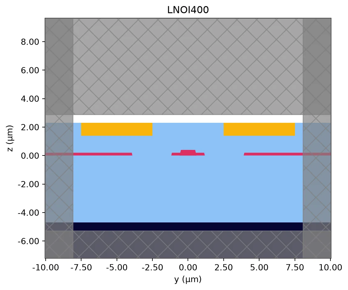

Crystal anisotropy

Lithium niobate is uniaxial: light polarized along the crystal $c$ axis sees the extraordinary index $n_e \approx 2.14$ , and light polarized across it sees the ordinary index $n_o \approx 2.21$ . In an x-cut film the $c$ axis lies in the plane of the chip, along $y$ in this PDK. A TE mode travelling along $x$ is polarized along $y$ , so it sees $n_e$ and the largest electro-optic coefficient, $r_{33}$ . This is why the modulators run along $x$ . The same TE mode travelling along $y$ sees $n_o$ , and the TM mode, polarized out of the plane, sees $n_o$ in either direction.

The cell below solves the 1 um ridge waveguide of the PDK for its first two modes in both directions. It also shows what this means for the rotator-combiner. A rotator converts TM0 into TE1 where the two modes have the same index, which is a question about the ridge width along the direction the device runs. The transmitter page designs the rotator-combiner along $x$ .

# Two modes of the single-mode ridge: TE0 and the TM0 the rotator-combiner works with
ridge = tech_tx.ports["RWG1000"].copy()
ridge.num_modes = 2

# The same cross-section facing +x and facing +y
modes = pf.port_modes(
    [pf.Port((0, 0), 180, ridge), pf.Port((0, 0), 270, ridge)],
    [f0],
    group_index=True,
    technology=tech_tx,
    verbose=False,
    show_progress=False,
)
for direction, ms in zip(("along x", "along y"), modes):
    n_eff = ms.data.n_eff.values.ravel()
    n_group = ms.data.n_group.values.ravel()
    te = ms.data.pol_fraction.te.values.ravel()
    for k in range(2):
        label = "TE" if te[k] > 0.5 else "TM"
        print(
            f"{direction}: mode {k} ({label}, TE fraction {te[k]:.2f})  "
            f"n_eff {n_eff[k]:.4f}  n_group {n_group[k]:.4f}"
        )

along x: mode 0 (TE, TE fraction 1.00)  n_eff 1.7915  n_group 2.1898
along x: mode 1 (TM, TE fraction 0.05)  n_eff 1.7104  n_group 2.2819
along y: mode 0 (TE, TE fraction 1.00)  n_eff 1.8524  n_group 2.2881
along y: mode 1 (TE, TE fraction 0.66)  n_eff 1.7141  n_group 2.1868

The TE index changes by about 0.06 between the two directions, which is the difference between $n_o$ and $n_e$ weighted by the fraction of the mode in the film. The TM index barely changes. Along $y$ the second mode is no longer a clean TM mode: in that direction its index nearly equals that of the TE mode family, and the slanted sidewalls of the ridge couple the two polarizations. The rotator-combiner relies on exactly this kind of hybridization, but at a controlled point along a taper. Along $x$ the two modes stay pure in the 1 um ridge, which is why the rotator-combiner is drawn along $x$ as well.

The group index of the TE mode along $x$ is the optical index that the travelling-wave electrode has to match with its microwave index, which the transmitter page uses.

Receiver technology

The receiver has no foundry PDK in this series, so this page writes one: a generic 220 nm SOI stack with a full and a partial silicon etch, germanium for the photodiodes, implants to contact them, a TiN heater layer and one aluminium routing metal. The structure follows the technology of the Optical I/O series, with two changes for this receiver.

The buried oxide is 3 um thick. The edge coupler of the receiver page is a subwavelength grating after Cheben et al. [4]. It expands the mode to match a high numerical aperture fiber, and the expanded mode would leak into the silicon substrate through a thinner oxide.
The germanium is 160 nm thick. It is the lateral p-i-n photodiode of Chen et al. [5], whose germanium is a 500 nm wide, 160 nm thick strip on the silicon, contacted through the silicon underneath. The p and n implants under the germanium, the p++ and n++ contact implants and a 120 nm polysilicon layer for its input taper are part of the stack for this reason.

Heights are measured from the bottom of the silicon device layer.

Level	z (um)	Material
Handle wafer	below -3.0	Si
Buried oxide	-3.0 to 0	SiO2
Silicon core	0 to 0.22	Si
Partial-etch slab	0 to 0.09	Si
Germanium	0.22 to 0.38	Ge
Polysilicon	0.22 to 0.34	Si
TiN heater	1.02 to 1.14	TiN
M1 routing	1.60 to 3.60	Al
Air	above 3.60	air

The edge-coupler facet is a deep trench etched through the whole stack, so the fiber faces the waveguide across air. The "Deep Trench" layer draws it.

Materials

Each material is a dictionary with an "optical" entry and an "electrical" entry. PhotonForge uses the first for mode solving and FDTD, and the second when the layout is extruded for a heat or charge simulation. The electrical entry is a MultiPhysicsMedium. The silicon entries carry a semiconductor model with doping, because the receiver page solves the photodiode junction with the charge solver: its capacitance and its depletion set the bandwidth.

# Silicon carrier model: band structure and Caughey-Thomas mobilities (cm^2/(V s)) for the charge solver
si_charge = td.SemiconductorMedium(
    permittivity=11.7,
    N_c=2.86e19,
    N_v=3.1e19,
    E_g=1.11,
    mobility_n=td.CaugheyThomasMobility(
        mu_min=52.2,
        mu=1471.0,
        ref_N=9.68e16,
        exp_N=0.68,
        exp_1=-0.57,
        exp_2=-2.33,
        exp_3=2.4,
        exp_4=-0.146,
    ),
    mobility_p=td.CaugheyThomasMobility(
        mu_min=44.9,
        mu=470.5,
        ref_N=2.23e17,
        exp_N=0.719,
        exp_1=-0.57,
        exp_2=-2.33,
        exp_3=2.4,
        exp_4=-0.146,
    ),
)
# Thermal properties: conductivity W/(um K), capacity J/(kg K), density kg/um^3
si_heat = td.SolidSpec(conductivity=148e-6, capacity=711, density=2.33e-15)

# One silicon entry per doping level: the optical model is the same for all of them
def silicon(name, n_a=None, n_d=None):
    charge = si_charge
    if n_a is not None:
        charge = charge.updated_copy(N_a=[td.ConstantDoping(concentration=n_a)])
    if n_d is not None:
        charge = charge.updated_copy(N_d=[td.ConstantDoping(concentration=n_d)])
    return {
        "optical": td.material_library["cSi"]["Li1993_293K"],
        "electrical": td.MultiPhysicsMedium(
            optical=td.Medium(permittivity=11.7), heat=si_heat, charge=charge, name=name
        ),
    }

si = silicon("Si")
# Junction implants of the photodiode (1e18 cm^-3) and the ohmic contact implants (1e20 cm^-3)
si_p = silicon("Si p", n_a=1e18)
si_n = silicon("Si n", n_d=1e18)
si_pp = silicon("Si p++", n_a=1e20)
si_nn = silicon("Si n++", n_d=1e20)

# Buried oxide and cladding
sio2 = {
    "optical": td.material_library["SiO2"]["Palik_Lossless"],
    "electrical": td.MultiPhysicsMedium(
        optical=td.Medium(permittivity=3.9),
        heat=td.SolidSpec(conductivity=1.38e-6, capacity=740, density=2.2e-15),
        charge=td.ChargeInsulatorMedium(permittivity=3.9),
        name="SiO2",
    ),
}

# Germanium absorber of the photodiodes, with its absorption at 1550 nm in the optical model.
# Undoped and fully depleted at reverse bias, it is a dielectric for the charge solver.
ge = {
    "optical": td.material_library["Ge"]["Icenogle1976"],
    "electrical": td.MultiPhysicsMedium(
        optical=td.Medium(permittivity=16.0),
        heat=td.SolidSpec(conductivity=60e-6, capacity=320, density=5.32e-15),
        charge=td.ChargeInsulatorMedium(permittivity=16.0),
        name="Ge",
    ),
}

# Heater metal. n and k are representative of a sputtered TiN film at 1550 nm.
tin = {
    "optical": td.medium_from_nk(n=2.6, k=4.2, freq=f0),
    "electrical": td.MultiPhysicsMedium(
        optical=td.PECMedium(),
        heat=td.SolidSpec(conductivity=29e-6, capacity=545, density=5.4e-15),
        charge=td.ChargeConductorMedium(conductivity=2.3),  # S/um
        name="TiN",
    ),
}

# Routing metal and the tungsten plugs that reach it
al = {
    "optical": td.material_library["Al"]["Rakic1995"],
    "electrical": td.MultiPhysicsMedium(
        optical=td.PECMedium(),
        heat=td.SolidSpec(conductivity=237e-6, capacity=900, density=2.7e-15),
        charge=td.ChargeConductorMedium(conductivity=38),
        name="Al",
    ),
}
w = {
    "optical": td.material_library["W"]["RakicLorentzDrude1998"],
    "electrical": td.MultiPhysicsMedium(
        optical=td.PECMedium(),
        heat=td.SolidSpec(conductivity=174e-6, capacity=132, density=19.3e-15),
        charge=td.ChargeConductorMedium(conductivity=18),
        name="W",
    ),
}

# Air above the cladding and in the facet trench
air = {
    "optical": td.Medium(permittivity=1),
    "electrical": td.MultiPhysicsMedium(
        optical=td.Medium(permittivity=1),
        heat=td.FluidSpec(),
        charge=td.ChargeInsulatorMedium(permittivity=1),
        name="Air",
    ),
}

The technology

Layers are the mask levels a designer draws on. The numbers follow the Optical I/O platform, so a cell drawn for one extrudes on the other.

Extrusion rules turn each mask into a material over a range in $z$ , and a later rule overrides an earlier one where they overlap. Two blanket rules come first: the handle wafer below $z = 0$ and the oxide from the bottom of the buried oxide to the top of the cladding. The silicon is cut into the oxide by the next rules: whatever is drawn on "Si" is 220 nm thick, and whatever is drawn on "Si Slab" but not on "Si" is the 90 nm slab. Each implant replaces the silicon it covers with a doped copy, in the core and in the slab. Germanium and polysilicon only grow where there is silicon underneath, so their masks are intersected with "Si".

Ports are the waveguide cross-sections. The 500 nm strip carries the receiver’s optical routing. It has a single-mode TE version and a version with both TE0 and TM0, which the PSR input needs. The rib, a 500 nm ridge on a 5 um slab, is the cross-section of the photodiode input.

Wrapping the definition in parametric_technology makes every stack dimension a keyword argument.

@pf.parametric_technology
def coherent_rx_soi(
    *,
    core_thickness=0.22,
    slab_thickness=0.09,  # silicon left by the partial etch
    box_thickness=3.0,  # buried oxide, thick enough for the expanded edge-coupler mode
    ge_thickness=0.16,
    poly_thickness=0.12,  # polysilicon of the photodiode input taper
    heater_separation=0.8,  # oxide between the silicon top and the heater
    heater_thickness=0.12,
    metal_separation=0.46,  # oxide between the heater top and M1
    metal_thickness=2.0,
    core_width=0.5,
    slab_width=5.0,
    si=si,
    si_p=si_p,
    si_n=si_n,
    si_pp=si_pp,
    si_nn=si_nn,
    sio2=sio2,
    ge=ge,
    tin=tin,
    al=al,
    w=w,
    air=air,
):
    layers = {
        "Si": pf.LayerSpec(
            (1, 0),
            description="Silicon, full thickness",
            color="#1f4e7918",
            pattern="/",
        ),
        "Si Slab": pf.LayerSpec(
            (2, 0),
            description="Silicon, partial etch to a 90 nm slab",
            color="#4f8fc018",
            pattern="\\",
        ),
        "Si p": pf.LayerSpec(
            (3, 0), description="P implant (photodiode)", color="#c8385a18", pattern="."
        ),
        "Si n": pf.LayerSpec(
            (4, 0), description="N implant (photodiode)", color="#3aa59618", pattern="."
        ),
        "Si p++": pf.LayerSpec(
            (5, 0), description="P++ ohmic implant", color="#8b1c3818", pattern="x"
        ),
        "Si n++": pf.LayerSpec(
            (6, 0), description="N++ ohmic implant", color="#1c6b6118", pattern="x"
        ),
        "Ge": pf.LayerSpec(
            (7, 0), description="Germanium detector", color="#7a5c9918", pattern="+"
        ),
        "Poly Si": pf.LayerSpec(
            (8, 0), description="Polysilicon on silicon", color="#2e8b5718", pattern="/"
        ),
        "Contact": pf.LayerSpec(
            (10, 0),
            description="Tungsten plug on silicon",
            color="#88888818",
            pattern="solid",
        ),
        "Ge Contact": pf.LayerSpec(
            (11, 0),
            description="Tungsten plug on germanium",
            color="#66666618",
            pattern="solid",
        ),
        "Heater": pf.LayerSpec(
            (12, 0), description="TiN heater", color="#d4a01718", pattern="-"
        ),
        "Via": pf.LayerSpec(
            (13, 0),
            description="Via from heater to M1",
            color="#aaaaaa18",
            pattern="solid",
        ),
        "M1": pf.LayerSpec(
            (14, 0),
            description="Aluminium routing metal",
            color="#b0b0b018",
            pattern="solid",
        ),
        # Mask only: the cladding ends at the top of M1, so the opening needs no extrusion rule
        "Pad Open": pf.LayerSpec(
            (15, 0), description="Passivation opening", color="#00000018", pattern=":"
        ),
        "Deep Trench": pf.LayerSpec(
            (16, 0),
            description="Deep trench at the edge-coupler facet",
            color="#ffffff18",
            pattern=".",
        ),
        # Drawing layer, on no mask: the chip area, which the design rule check reads
        "FloorPlan": pf.LayerSpec(
            (99, 0), description="Chip area", color="#2e7d5b10", pattern="hollow"
        ),
    }

    # z = 0 is the bottom of the silicon device layer.
    z_ge = core_thickness + ge_thickness
    z_heater = core_thickness + heater_separation
    z_metal = z_heater + heater_thickness + metal_separation
    core = pf.MaskSpec((1, 0))
    slab = pf.MaskSpec((2, 0)) - core

    extrusion_specs = [
        # Blanket rules first, no mask: the handle wafer and the oxide. Each has one limit
        # at a finite height, and the oxide overwrites the wafer above the buried-oxide floor.
        pf.ExtrusionSpec(pf.MaskSpec(), si, (-pf.Z_INF, 0)),
        pf.ExtrusionSpec(
            pf.MaskSpec(), sio2, (-box_thickness, z_metal + metal_thickness)
        ),
        pf.ExtrusionSpec(core, si, (0, core_thickness)),
        pf.ExtrusionSpec(slab, si, (0, slab_thickness)),
    ]

    # Each implant replaces the silicon it covers, in the core and in the slab
    for layer, medium in (
        ((3, 0), si_p),
        ((4, 0), si_n),
        ((5, 0), si_pp),
        ((6, 0), si_nn),
    ):
        implant = pf.MaskSpec(layer)
        extrusion_specs.append(
            pf.ExtrusionSpec(implant * core, medium, (0, core_thickness))
        )
        extrusion_specs.append(
            pf.ExtrusionSpec(implant * slab, medium, (0, slab_thickness))
        )

    extrusion_specs += [
        # Germanium and polysilicon grow on the full-thickness silicon only
        pf.ExtrusionSpec(pf.MaskSpec((7, 0)) * core, ge, (core_thickness, z_ge)),
        # The optical model uses crystalline silicon for the polysilicon
        pf.ExtrusionSpec(
            pf.MaskSpec((8, 0)) * core,
            si,
            (core_thickness, core_thickness + poly_thickness),
        ),
        # Plugs land on the full-thickness silicon, which the receiver rule deck requires,
        # and run from its top up to the bottom of M1
        pf.ExtrusionSpec(pf.MaskSpec((10, 0)), w, (core_thickness, z_metal)),
        pf.ExtrusionSpec(pf.MaskSpec((11, 0)), w, (z_ge, z_metal)),
        pf.ExtrusionSpec(
            pf.MaskSpec((12, 0)), tin, (z_heater, z_heater + heater_thickness)
        ),
        pf.ExtrusionSpec(
            pf.MaskSpec((13, 0)), w, (z_heater + heater_thickness, z_metal)
        ),
        pf.ExtrusionSpec(
            pf.MaskSpec((14, 0)), al, (z_metal, z_metal + metal_thickness)
        ),
        # The facet trench cuts through everything, so it comes last
        pf.ExtrusionSpec(pf.MaskSpec((16, 0)), air, (-pf.Z_INF, pf.Z_INF)),
    ]

    ports = {
        "Strip_TE": pf.PortSpec(
            description="Strip waveguide, TE, 500 nm",
            width=3.0,  # simulation window, wide enough for the evanescent tail
            limits=(-1.0, 1.22),
            num_modes=1,
            target_neff=3.5,  # the core index, a search hint for the mode solver
            path_profiles=[(core_width, 0, (1, 0))],
        ),
        "Strip_TE_TM": pf.PortSpec(
            description="Strip waveguide, TE0 and TM0, 500 nm",
            width=3.0,
            limits=(-1.0, 1.22),
            num_modes=2,
            target_neff=3.5,
            path_profiles=[(core_width, 0, (1, 0))],
        ),
        "Rib_TE": pf.PortSpec(
            description="Rib waveguide on a 90 nm slab, TE, 500 nm",
            width=4.0,  # narrower than the drawn slab, so any wider slab matches too
            limits=(-1.0, 1.22),
            num_modes=1,
            target_neff=3.5,
            path_profiles=[(core_width, 0, (1, 0)), (slab_width, 0, (2, 0))],
        ),
    }

    return pf.Technology(
        name="Coherent RX SOI",
        version="1.0",
        layers=layers,
        extrusion_specs=extrusion_specs,
        ports=ports,
        # Air everywhere that no rule fills: above the cladding and beyond the chip
        background_medium=air,
    )

tech_rx = coherent_rx_soi()
tech_rx.layers

Name	Layer	Description	Color	Pattern
Si	(1, 0)	Silicon, full thickness	#1f4e7918	/
Si Slab	(2, 0)	Silicon, partial etch to a 90… … nm slab	#4f8fc018	\
Si p	(3, 0)	P implant (photodiode)	#c8385a18	.
Si n	(4, 0)	N implant (photodiode)	#3aa59618	.
Si p++	(5, 0)	P++ ohmic implant	#8b1c3818	x
Si n++	(6, 0)	N++ ohmic implant	#1c6b6118	x
Ge	(7, 0)	Germanium detector	#7a5c9918	+
Poly Si	(8, 0)	Polysilicon on silicon	#2e8b5718	/
Contact	(10, 0)	Tungsten plug on silicon	#88888818	solid
Ge Contact	(11, 0)	Tungsten plug on germanium	#66666618	solid
Heater	(12, 0)	TiN heater	#d4a01718	-
Via	(13, 0)	Via from heater to M1	#aaaaaa18	solid
M1	(14, 0)	Aluminium routing metal	#b0b0b018	solid
Pad Open	(15, 0)	Passivation opening	#00000018	:
Deep Trench	(16, 0)	Deep trench at the edge-coupler… … facet	#ffffff18	.
FloorPlan	(99, 0)	Chip area	#2e7d5b10	hollow

# The rule that turns each drawing layer into a solid, with its z extent and medium
tech_rx.extrusion_specs

#	Mask	Limits (μm)	Opt. Medium	Elec. Medium
0	()	-inf, 0	cSi_Li1993_293K	MultiPhysicsMedium(name='Si',… … optical={'permittivity': 11.7}, heat={'capacity': 711.0, 'conductivity': 0.000148, 'density': 2.33e-15}, charge={'permittivity': 11.7, 'N_c': {'N': 2.86e+19}, 'N_v': {'N': 3.1e+19}, 'E_g': {'eg': 1.11}, 'mobility_n': {'mu_min': 52.2, 'mu': 1471.0, 'exp_2': -2.33, 'exp_N': 0.68, 'ref_N': 9.68e+16, 'exp_1': -0.57, 'exp_3': 2.4, 'exp_4': -0.146}, 'mobility_p': {'mu_min': 44.9, 'mu': 470.5, 'exp_2': -2.33, 'exp_N': 0.719, 'ref_N': 2.23e+17, 'exp_1': -0.57, 'exp_3': 2.4, 'exp_4': -0.146}})
1	()	-3, 3.6	SiO2_Palik_LowLoss	MultiPhysicsMedium(name='SiO2',… … optical={'permittivity': 3.9}, heat={'capacity': 740.0, 'conductivity': 1.38e-06, 'density': 2.2e-15}, charge={'permittivity': 3.9})
2	'Si'	0, 0.22	cSi_Li1993_293K	MultiPhysicsMedium(name='Si',… … optical={'permittivity': 11.7}, heat={'capacity': 711.0, 'conductivity': 0.000148, 'density': 2.33e-15}, charge={'permittivity': 11.7, 'N_c': {'N': 2.86e+19}, 'N_v': {'N': 3.1e+19}, 'E_g': {'eg': 1.11}, 'mobility_n': {'mu_min': 52.2, 'mu': 1471.0, 'exp_2': -2.33, 'exp_N': 0.68, 'ref_N': 9.68e+16, 'exp_1': -0.57, 'exp_3': 2.4, 'exp_4': -0.146}, 'mobility_p': {'mu_min': 44.9, 'mu': 470.5, 'exp_2': -2.33, 'exp_N': 0.719, 'ref_N': 2.23e+17, 'exp_1': -0.57, 'exp_3': 2.4, 'exp_4': -0.146}})
3	'Si Slab' - 'Si'	0, 0.09	cSi_Li1993_293K	MultiPhysicsMedium(name='Si',… … optical={'permittivity': 11.7}, heat={'capacity': 711.0, 'conductivity': 0.000148, 'density': 2.33e-15}, charge={'permittivity': 11.7, 'N_c': {'N': 2.86e+19}, 'N_v': {'N': 3.1e+19}, 'E_g': {'eg': 1.11}, 'mobility_n': {'mu_min': 52.2, 'mu': 1471.0, 'exp_2': -2.33, 'exp_N': 0.68, 'ref_N': 9.68e+16, 'exp_1': -0.57, 'exp_3': 2.4, 'exp_4': -0.146}, 'mobility_p': {'mu_min': 44.9, 'mu': 470.5, 'exp_2': -2.33, 'exp_N': 0.719, 'ref_N': 2.23e+17, 'exp_1': -0.57, 'exp_3': 2.4, 'exp_4': -0.146}})
4	'Si p' * 'Si'	0, 0.22	cSi_Li1993_293K	MultiPhysicsMedium(name='Si p',… … optical={'permittivity': 11.7}, heat={'capacity': 711.0, 'conductivity': 0.000148, 'density': 2.33e-15}, charge={'permittivity': 11.7, 'N_c': {'N': 2.86e+19}, 'N_v': {'N': 3.1e+19}, 'E_g': {'eg': 1.11}, 'mobility_n': {'mu_min': 52.2, 'mu': 1471.0, 'exp_2': -2.33, 'exp_N': 0.68, 'ref_N': 9.68e+16, 'exp_1': -0.57, 'exp_3': 2.4, 'exp_4': -0.146}, 'mobility_p': {'mu_min': 44.9, 'mu': 470.5, 'exp_2': -2.33, 'exp_N': 0.719, 'ref_N': 2.23e+17, 'exp_1': -0.57, 'exp_3': 2.4, 'exp_4': -0.146}, 'N_a': ({'concentration': 1e+18},)})
5	'Si p' * ('Si Slab' - 'Si')	0, 0.09	cSi_Li1993_293K	MultiPhysicsMedium(name='Si p',… … optical={'permittivity': 11.7}, heat={'capacity': 711.0, 'conductivity': 0.000148, 'density': 2.33e-15}, charge={'permittivity': 11.7, 'N_c': {'N': 2.86e+19}, 'N_v': {'N': 3.1e+19}, 'E_g': {'eg': 1.11}, 'mobility_n': {'mu_min': 52.2, 'mu': 1471.0, 'exp_2': -2.33, 'exp_N': 0.68, 'ref_N': 9.68e+16, 'exp_1': -0.57, 'exp_3': 2.4, 'exp_4': -0.146}, 'mobility_p': {'mu_min': 44.9, 'mu': 470.5, 'exp_2': -2.33, 'exp_N': 0.719, 'ref_N': 2.23e+17, 'exp_1': -0.57, 'exp_3': 2.4, 'exp_4': -0.146}, 'N_a': ({'concentration': 1e+18},)})
6	'Si n' * 'Si'	0, 0.22	cSi_Li1993_293K	MultiPhysicsMedium(name='Si n',… … optical={'permittivity': 11.7}, heat={'capacity': 711.0, 'conductivity': 0.000148, 'density': 2.33e-15}, charge={'permittivity': 11.7, 'N_c': {'N': 2.86e+19}, 'N_v': {'N': 3.1e+19}, 'E_g': {'eg': 1.11}, 'mobility_n': {'mu_min': 52.2, 'mu': 1471.0, 'exp_2': -2.33, 'exp_N': 0.68, 'ref_N': 9.68e+16, 'exp_1': -0.57, 'exp_3': 2.4, 'exp_4': -0.146}, 'mobility_p': {'mu_min': 44.9, 'mu': 470.5, 'exp_2': -2.33, 'exp_N': 0.719, 'ref_N': 2.23e+17, 'exp_1': -0.57, 'exp_3': 2.4, 'exp_4': -0.146}, 'N_d': ({'concentration': 1e+18},)})
7	'Si n' * ('Si Slab' - 'Si')	0, 0.09	cSi_Li1993_293K	MultiPhysicsMedium(name='Si n',… … optical={'permittivity': 11.7}, heat={'capacity': 711.0, 'conductivity': 0.000148, 'density': 2.33e-15}, charge={'permittivity': 11.7, 'N_c': {'N': 2.86e+19}, 'N_v': {'N': 3.1e+19}, 'E_g': {'eg': 1.11}, 'mobility_n': {'mu_min': 52.2, 'mu': 1471.0, 'exp_2': -2.33, 'exp_N': 0.68, 'ref_N': 9.68e+16, 'exp_1': -0.57, 'exp_3': 2.4, 'exp_4': -0.146}, 'mobility_p': {'mu_min': 44.9, 'mu': 470.5, 'exp_2': -2.33, 'exp_N': 0.719, 'ref_N': 2.23e+17, 'exp_1': -0.57, 'exp_3': 2.4, 'exp_4': -0.146}, 'N_d': ({'concentration': 1e+18},)})
8	'Si p++' * 'Si'	0, 0.22	cSi_Li1993_293K	MultiPhysicsMedium(name='Si… … p++', optical={'permittivity': 11.7}, heat={'capacity': 711.0, 'conductivity': 0.000148, 'density': 2.33e-15}, charge={'permittivity': 11.7, 'N_c': {'N': 2.86e+19}, 'N_v': {'N': 3.1e+19}, 'E_g': {'eg': 1.11}, 'mobility_n': {'mu_min': 52.2, 'mu': 1471.0, 'exp_2': -2.33, 'exp_N': 0.68, 'ref_N': 9.68e+16, 'exp_1': -0.57, 'exp_3': 2.4, 'exp_4': -0.146}, 'mobility_p': {'mu_min': 44.9, 'mu': 470.5, 'exp_2': -2.33, 'exp_N': 0.719, 'ref_N': 2.23e+17, 'exp_1': -0.57, 'exp_3': 2.4, 'exp_4': -0.146}, 'N_a': ({'concentration': 1e+20},)})
9	'Si p++' * ('Si Slab' - 'Si')	0, 0.09	cSi_Li1993_293K	MultiPhysicsMedium(name='Si… … p++', optical={'permittivity': 11.7}, heat={'capacity': 711.0, 'conductivity': 0.000148, 'density': 2.33e-15}, charge={'permittivity': 11.7, 'N_c': {'N': 2.86e+19}, 'N_v': {'N': 3.1e+19}, 'E_g': {'eg': 1.11}, 'mobility_n': {'mu_min': 52.2, 'mu': 1471.0, 'exp_2': -2.33, 'exp_N': 0.68, 'ref_N': 9.68e+16, 'exp_1': -0.57, 'exp_3': 2.4, 'exp_4': -0.146}, 'mobility_p': {'mu_min': 44.9, 'mu': 470.5, 'exp_2': -2.33, 'exp_N': 0.719, 'ref_N': 2.23e+17, 'exp_1': -0.57, 'exp_3': 2.4, 'exp_4': -0.146}, 'N_a': ({'concentration': 1e+20},)})
10	'Si n++' * 'Si'	0, 0.22	cSi_Li1993_293K	MultiPhysicsMedium(name='Si… … n++', optical={'permittivity': 11.7}, heat={'capacity': 711.0, 'conductivity': 0.000148, 'density': 2.33e-15}, charge={'permittivity': 11.7, 'N_c': {'N': 2.86e+19}, 'N_v': {'N': 3.1e+19}, 'E_g': {'eg': 1.11}, 'mobility_n': {'mu_min': 52.2, 'mu': 1471.0, 'exp_2': -2.33, 'exp_N': 0.68, 'ref_N': 9.68e+16, 'exp_1': -0.57, 'exp_3': 2.4, 'exp_4': -0.146}, 'mobility_p': {'mu_min': 44.9, 'mu': 470.5, 'exp_2': -2.33, 'exp_N': 0.719, 'ref_N': 2.23e+17, 'exp_1': -0.57, 'exp_3': 2.4, 'exp_4': -0.146}, 'N_d': ({'concentration': 1e+20},)})
11	'Si n++' * ('Si Slab' - 'Si')	0, 0.09	cSi_Li1993_293K	MultiPhysicsMedium(name='Si… … n++', optical={'permittivity': 11.7}, heat={'capacity': 711.0, 'conductivity': 0.000148, 'density': 2.33e-15}, charge={'permittivity': 11.7, 'N_c': {'N': 2.86e+19}, 'N_v': {'N': 3.1e+19}, 'E_g': {'eg': 1.11}, 'mobility_n': {'mu_min': 52.2, 'mu': 1471.0, 'exp_2': -2.33, 'exp_N': 0.68, 'ref_N': 9.68e+16, 'exp_1': -0.57, 'exp_3': 2.4, 'exp_4': -0.146}, 'mobility_p': {'mu_min': 44.9, 'mu': 470.5, 'exp_2': -2.33, 'exp_N': 0.719, 'ref_N': 2.23e+17, 'exp_1': -0.57, 'exp_3': 2.4, 'exp_4': -0.146}, 'N_d': ({'concentration': 1e+20},)})
12	'Ge' * 'Si'	0.22, 0.38	Ge_Icenogle1976	MultiPhysicsMedium(name='Ge',… … optical={'permittivity': 16.0}, heat={'capacity': 320.0, 'conductivity': 6e-05, 'density': 5.32e-15}, charge={'permittivity': 16.0})
13	'Poly Si' * 'Si'	0.22, 0.34	cSi_Li1993_293K	MultiPhysicsMedium(name='Si',… … optical={'permittivity': 11.7}, heat={'capacity': 711.0, 'conductivity': 0.000148, 'density': 2.33e-15}, charge={'permittivity': 11.7, 'N_c': {'N': 2.86e+19}, 'N_v': {'N': 3.1e+19}, 'E_g': {'eg': 1.11}, 'mobility_n': {'mu_min': 52.2, 'mu': 1471.0, 'exp_2': -2.33, 'exp_N': 0.68, 'ref_N': 9.68e+16, 'exp_1': -0.57, 'exp_3': 2.4, 'exp_4': -0.146}, 'mobility_p': {'mu_min': 44.9, 'mu': 470.5, 'exp_2': -2.33, 'exp_N': 0.719, 'ref_N': 2.23e+17, 'exp_1': -0.57, 'exp_3': 2.4, 'exp_4': -0.146}})
14	'Contact'	0.22, 1.6	W_RakicLorentzDrude1998	MultiPhysicsMedium(name='W',… … optical={}, heat={'capacity': 132.0, 'conductivity': 0.000174, 'density': 1.93e-14}, charge={'conductivity': 18.0})
15	'Ge Contact'	0.38, 1.6	W_RakicLorentzDrude1998	MultiPhysicsMedium(name='W',… … optical={}, heat={'capacity': 132.0, 'conductivity': 0.000174, 'density': 1.93e-14}, charge={'conductivity': 18.0})
16	'Heater'	1.02, 1.14	Lorentz(coeffs=… …((21.840000000000003, 162323815372577.7, 52562735135327.414),))	MultiPhysicsMedium(name='TiN',… … optical={}, heat={'capacity': 545.0, 'conductivity': 2.9e-05, 'density': 5.4e-15}, charge={'conductivity': 2.3})
17	'Via'	1.14, 1.6	W_RakicLorentzDrude1998	MultiPhysicsMedium(name='W',… … optical={}, heat={'capacity': 132.0, 'conductivity': 0.000174, 'density': 1.93e-14}, charge={'conductivity': 18.0})
18	'M1'	1.6, 3.6	Al_Rakic1995	MultiPhysicsMedium(name='Al',… … optical={}, heat={'capacity': 900.0, 'conductivity': 0.000237, 'density': 2.7e-15}, charge={'conductivity': 38.0})
19	'Deep Trench'	-inf, inf	Medium()	MultiPhysicsMedium(name='Air',… … optical={}, heat={}, charge={})

# The waveguide cross-sections available as ports
tech_rx.ports

Name	Classification	Description	Width (μm)	Limits (μm)	Modes	Target n_eff	Path profiles (μm)
Rib_TE	optical	Rib waveguide on a 90 nm slab,… … TE, 500 nm	4	-1, 1.22	1	3.5	'Si': 0.5, 'Si Slab': 5
Strip_TE	optical	Strip waveguide, TE, 500 nm	3	-1, 1.22	1	3.5	'Si': 0.5
Strip_TE_TM	optical	Strip waveguide, TE0 and TM0,… … 500 nm	3	-1, 1.22	2	3.5	'Si': 0.5

Cross-section check

A test cell with one shape per rule is the direct check of the extrusion rules. It holds a strip waveguide under a heater with its via and M1 feed, a rib waveguide, and a cut through the photodiode: the germanium strip on the silicon, the p and n implants meeting under its centre, the contact implants at the two sides with a tungsten plug on each, and the polysilicon of the input taper. A deep trench ends the cell on the left, as it ends the chip at the edge coupler.

pd_half_width = 2.2  # Silicon under and beside the germanium, each side (um)
contact_offset = 1.2  # Inner edge of the contact implants (um)

xs = pf.Component("cross_section", technology=tech_rx)

# Strip waveguide along x at y = -6, with the heater above it and an M1 feed on the via
xs.add("Si", pf.Rectangle((-4, -6.25), (4, -5.75)))
xs.add("Heater", pf.Rectangle((-4, -6.5), (4, -5.5)))
xs.add(
    "Via",
    pf.Rectangle((2.5, -6.4), (3.5, -5.6)),
    "M1",
    pf.Rectangle((2.5, -7.5), (4, -4.5)),
)

# Rib waveguide at y = 0: the strip on a 5 um slab
xs.add(
    "Si",
    pf.Rectangle((-4, -0.25), (4, 0.25)),
    "Si Slab",
    pf.Rectangle((-4, -2.5), (4, 2.5)),
)

# Photodiode at y = 7: Ge on Si, junction implants under it, contact implants and plugs outside
y_pd = 7.0
xs.add(
    "Si",
    pf.Rectangle((-4, y_pd - pd_half_width), (4, y_pd + pd_half_width)),
    "Ge",
    pf.Rectangle((0, y_pd - 0.25), (4, y_pd + 0.25)),
    "Poly Si",
    pf.Rectangle((-4, y_pd - 0.1), (0, y_pd + 0.1)),
    "Si n",
    pf.Rectangle((0, y_pd - pd_half_width), (4, y_pd)),
    "Si p",
    pf.Rectangle((0, y_pd), (4, y_pd + pd_half_width)),
    "Si n++",
    pf.Rectangle((0, y_pd - pd_half_width), (4, y_pd - contact_offset)),
    "Si p++",
    pf.Rectangle((0, y_pd + contact_offset), (4, y_pd + pd_half_width)),
)
for sign in (-1, 1):
    y_plug = y_pd + sign * (contact_offset + pd_half_width) / 2
    xs.add("Contact", pf.Rectangle((1, y_plug - 0.2), (3, y_plug + 0.2)))
    xs.add("M1", pf.Rectangle((0.5, y_plug - 0.4), (3.5, y_plug + 0.4)))

# Deep trench at the left end
xs.add("Deep Trench", pf.Rectangle((-6, -8), (-4, 10)))

fig, ax = plt.subplots(
    1, 4, figsize=(18, 3.6), gridspec_kw={"width_ratios": [1, 1.6, 1.6, 1.4]}
)

# Across the strip: the core with the heater above it and the M1 feed on its via
pf.tidy3d_plot(xs, x=3, ax=ax[0], plot_type="structures", frequency=f0)
ax[0].set_xlim(-7.6, -4.4)
ax[0].set_ylim(-1.0, 4.0)
ax[0].set_title("strip under the heater")

# Across the rib: the core on its 90 nm slab
pf.tidy3d_plot(xs, x=0, ax=ax[1], plot_type="structures", frequency=f0)
ax[1].set_xlim(-2.8, 2.8)
ax[1].set_ylim(-0.6, 1.0)
ax[1].set_title("rib")

# Across the photodiode: germanium on silicon, contact plugs on the outer silicon
pf.tidy3d_plot(xs, x=2, ax=ax[2], plot_type="structures", frequency=f0)
ax[2].set_xlim(y_pd - 2.8, y_pd + 2.8)
ax[2].set_ylim(-0.6, 1.0)
ax[2].set_title("photodiode")

# Along the photodiode axis: polysilicon taper, germanium, and the facet trench through the stack
pf.tidy3d_plot(xs, y=y_pd, ax=ax[3], plot_type="structures", frequency=f0)
ax[3].set_xlim(-6.5, 4.5)
ax[3].set_ylim(-3.5, 4.2)
ax[3].set_title("along the photodiode")
plt.show()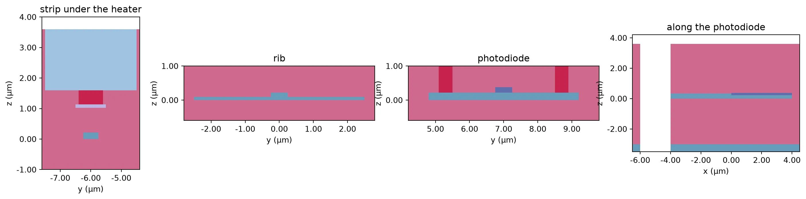

Waveguide modes

The strip carries both polarizations into the PSR, so the cell below solves its TE0 and TM0 modes along with the rib mode. The index difference between TE0 and TM0 is what a polarization rotator has to bridge, and the group indices set the skew between paths of the same length.

modes = pf.port_modes(
    ["Strip_TE_TM", "Rib_TE"],
    [f0],
    group_index=True,
    technology=tech_rx,
    verbose=False,
    show_progress=False,
)
for name, ms in zip(("strip", "rib"), modes):
    n_eff = ms.data.n_eff.values.ravel()
    n_group = ms.data.n_group.values.ravel()
    te = ms.data.pol_fraction.te.values.ravel()
    for k in range(len(n_eff)):
        label = "TE" if te[k] > 0.5 else "TM"
        print(f"{name} {label}0: n_eff {n_eff[k]:.4f}  n_group {n_group[k]:.4f}")

# Field of the two strip modes
fig, ax = plt.subplots(1, 2, figsize=(10, 3.2), tight_layout=True)
for k in range(2):
    modes[0].plot_field("E", mode_index=k, val="abs", ax=ax[k])
    ax[k].set_title(("TE0", "TM0")[k])
plt.show()

strip TE0: n_eff 2.4389  n_group 4.1777
strip TM0: n_eff 1.7800  n_group 3.7820
rib TE0: n_eff 2.5619  n_group 3.8800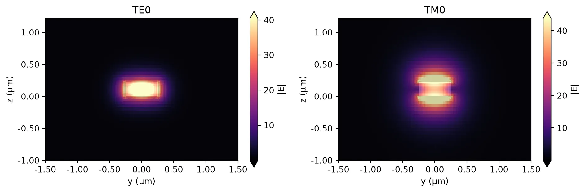

What comes next

Both technologies are in place. The transmitter page designs the travelling-wave modulator on LNOI400 and builds the rest of the transmitter library; the receiver page designs the receiver components on the SOI technology written here. Both pages attach a model to every component, and the link page simulates the two chips together from those models.