Resonance Locking

Download notebook (.zip)

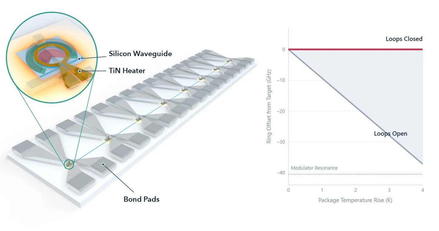
The chip the series arrives at, with the part this notebook works on marked:

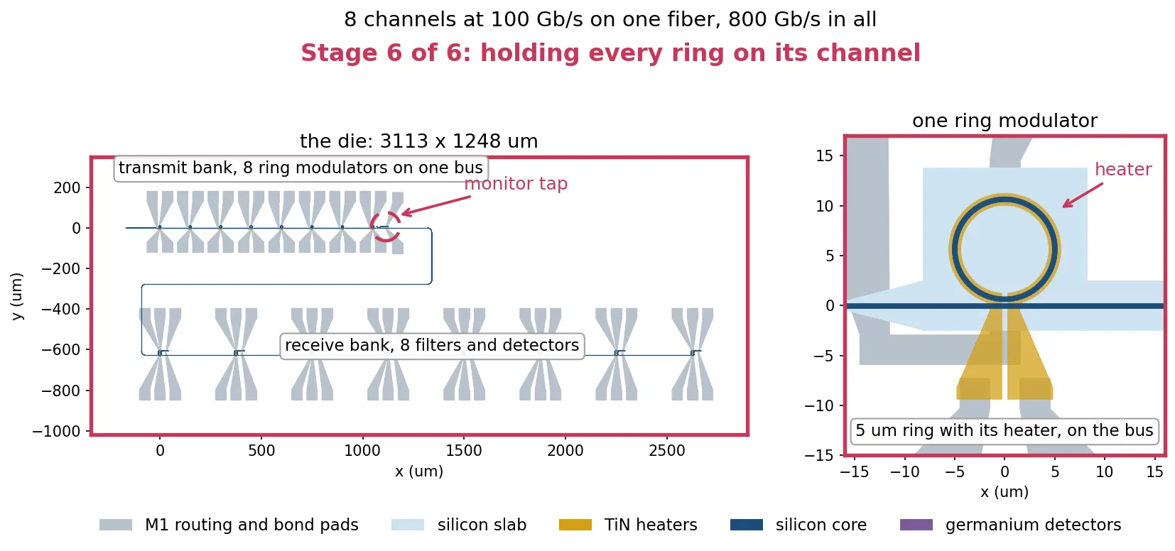
Wavelength Plan and Thermal Budget sets the power of every heater on the chip from a calibration made at one temperature. When the package temperature changes, every resonance moves: by 9.3 GHz per kelvin for the modulator rings. This is large compared with the two frequency differences that matter on this chip. The modulator operates about 40 GHz below its resonance, and the drop filter passband is about 140 GHz wide. A temperature change of a few kelvin therefore degrades the link, and each heater needs a feedback loop that corrects its power continuously. The chip has 24 heaters: one on each of the eight modulators and two on each of the eight drop filters.

A feedback loop needs an error signal: a measured quantity that is zero when the ring is at its target and changes sign when the ring moves to either side of it. A common way to obtain one is dithering [1, 2]: a small sinusoidal modulation is added to the heater power, and a lock-in amplifier measures how the photodiode current responds to it. The loop itself, from the lock-in amplifier to the integrator that sets the heater power, is shown for a single ring in Microring Thermal Stabilization. This page addresses what is specific to this chip. The two devices need different error signals, and neither is the standard case of a ring held at its transmission minimum [1].

The page covers:

• The heater: its thermal time constant, which limits the usable dither frequencies.
• The drop filter: two heaters per filter, and an error signal that works because the 100 Gb/s data fills the passband.
• The modulator: an error signal from the second harmonic of the dither, which holds the ring at its operating point regardless of the optical power on the shared monitor photodiode.
• All 24 loops together, with the package temperature changing, and eye diagrams with the loops open and closed.

References

1. Padmaraju, K., Logan, D. F., Shiraishi, T., Ackert, J. J., Knights, A. P., and Bergman, K. “Wavelength locking and thermally stabilizing microring resonators using dithering signals.” Journal of Lightwave Technology 2014 32 (3), 505-512, doi: 10.1109/JLT.2013.2294564.
2. Padmaraju, K., and Bergman, K. “Resolving the thermal challenges for silicon microring resonator devices.” Nanophotonics 2014 3 (4-5), 269-281, doi: 10.1515/nanoph-2013-0013.
3. Padmaraju, K., Chan, J., Chen, L., Lipson, M., and Bergman, K. “Thermal stabilization of a microring modulator using feedback control.” Optics Express 2012 20 (27), 27999-28008, doi: 10.1364/OE.20.027999.
4. Little, B. E., Chu, S. T., Haus, H. A., Foresi, J., and Laine, J.-P. “Microring resonator channel dropping filters.” Journal of Lightwave Technology 1997 15 (6), 998-1005, doi: 10.1109/50.588673.

from runpy import run_path

# Optical_IO_Chip.qmd defines what this notebook builds on: the cells and every measured
# number. Its shared cells are generated into the module below; see
# docs/scripts/generate_notebook_modules.py.
globals().update(
    {k: v for k, v in run_path("misc/optical_io_chip.py").items() if not k.startswith("_")}
)

Thermal constants and settings

The thermal results are read from misc/thermal_budget.npz, written by Wavelength Plan and Thermal Budget. Three of them are used throughout this page:

• the temperature rise of a ring per milliwatt of its heater power,
• the fraction of that rise that reaches a ring 150 um away,
• the spread of resonance frequencies between rings on the same die after fabrication.

The same file holds the dimensions of the thermal stack, so the HEAT simulations below use the same die. The temperature rise per milliwatt was measured on the modulator; the filter’s value is measured further below.

from photonforge.live_viewer import LiveViewer
from scipy.interpolate import RegularGridInterpolator
from tidy3d import web

# Open a layout viewer for the cells shown on this page
viewer = LiveViewer()

# We raise the Tidy3D logging level to reduce output noise from the solves
# below. Warnings can flag real problems, so only suppress them once you have
# confirmed they are not relevant to your case.
td.config.logging.level = "ERROR"

# Load the thermal results measured in Optical_IO_Thermal.ipynb
budget = np.load("misc/thermal_budget.npz")

# Ring temperature rise per milliwatt of its own heater (K/mW)
k_per_mw = float(budget["k_per_mw"])

# Fraction of a ring's temperature rise that reaches a ring 150 um away
coupling = float(budget["coupling"])

# Spread of resonance frequencies between rings on one die, one sigma (GHz)
sigma_ring = float(budget["differential"])

mean_mw = float(budget["mean_mw"])  # Average trim power per ring (mW)
worst_mw = float(budget["worst_mw"])  # Largest trim power on any ring (mW)

z_heater = float(budget["z_heater"])  # Height of the heater's lower face (um)
h_heater = float(budget["h_heater"])  # Heater thickness (um)
h_box = float(budget["h_box"])  # Buried oxide thickness (um)
clad_top = float(budget["clad_top"])  # Top of the oxide cladding (um)
die_thickness = float(budget["die_thickness"])  # Silicon die below the oxide (um)
lateral_pad = float(budget["lateral_pad"])  # Oxide added around each cell (um)

z_wg = tech.parametric_kwargs["core_thickness"] / 2  # Mid-core height (um)
air_margin = 2.0  # Air above and below the die (um)
p_probe = 1.0e-3  # Heater power used in the thermal simulations (W)
t_ref = 293.0  # Temperature the component models were built at (K)

# Convert the modulator heater's efficiency to a resonance shift
ghz_per_mw_rib = k_per_mw * ghz_per_k_rib

print(f"heater efficiency      {k_per_mw:.2f} K/mW")
print(f"modulator tuning       {ghz_per_k_rib:.2f} GHz/K = {ghz_per_mw_rib:.1f} GHz/mW")
print(f"filter tuning          {ghz_per_k_strip:.2f} GHz/K")
print(f"ring-to-ring spread    {sigma_ring:.1f} GHz, one sigma")
print(f"coupling at 150 um     {coupling:.1e}")

LiveViewer started at http://127.0.0.1:34103. Call its 'stop()' method to free the port.
heater efficiency      3.57 K/mW
modulator tuning       9.31 GHz/K = 33.2 GHz/mW
filter tuning          8.62 GHz/K
ring-to-ring spread    45.6 GHz, one sigma
coupling at 150 um     7.7e-05

Thermal time constant of the heater

The heater is a TiN track above the ring. When its power changes, heat must diffuse through the oxide before the ring temperature follows. The time to diffuse a distance $d$ through a material with thermal diffusivity $\alpha = \kappa / (\rho c_p)$ is about $d^2 / \alpha$, where $\kappa$ is the thermal conductivity, $\rho$ the density and $c_p$ the specific heat. The oxide sets this time, because silicon conducts heat about a hundred times better. The cell below evaluates this estimate for the distance from the heater to the silicon die.

# Calculate the oxide's thermal diffusivity from its conductivity and heat capacity
ox = sio2["electrical"].heat  # Thermal properties of the oxide
alpha_ox = ox.conductivity / (ox.density * ox.capacity)  # Diffusivity (um^2/s)

# Estimate the time for heat to diffuse from the heater to the silicon die
span_ox = z_heater + h_box  # Distance from the heater to the die (um)
tau_estimate = span_ox**2 / alpha_ox  # Diffusion time over that distance (s)

print(f"oxide diffusivity     {alpha_ox:.3g} um^2/s")
print(f"heater to die         {span_ox:.2f} um")
print(f"diffusion estimate    {tau_estimate*1e6:.1f} us")

oxide diffusivity     8.48e+05 um^2/s
heater to die         3.02 um
diffusion estimate    10.8 us

A transient HEAT simulation measures the time constant directly. Every structure in it comes from the layout:

• The modulator is extruded from its cell with Component.extrude, using the technology of the series, so the waveguide, implants, contacts, heater and metal are those of the drawn cell.
• The die and the cladding are drawn as one rectangle on the FloorPlan layer, around the cell. A copy of the technology adds two extrusion rules for this layer: silicon below the buried oxide, and oxide from the buried oxide to the top of the cladding.
• The heat source is drawn on a new layer, Heat Source, which the same copy extrudes in TiN over the full thickness of the heater. It covers only the narrow ring track of the heater. Electrical power is dissipated where the current density is high, which is in the narrow track; the wide feed carries the same current at a much lower density. A heat source spread uniformly over the whole drawn heater would put a large part of the power in the feed.

The heated volume, which converts the heater power into a heat source density, is the drawn area of the heated region times the heater thickness.

The plots show the model at the height of the heater and in a vertical cut through the ring centre.

# Modulator heater track width (um)
heater_width = mrm.parametric_kwargs["heater_width"]
heater_slot = mrm.parametric_kwargs["heater_slot"]  # Feed slot width (um)

inset = 0.05 * heater_width  # Gap from the heated annulus to the track edges (um)
arc_r_out = r_target + heater_width / 2 - inset  # Outer radius of heated annulus (um)
arc_r_in = r_target - heater_width / 2 + inset  # Inner radius of heated annulus (um)
z_mid = z_heater + h_heater / 2  # Mid-height of the heater (um)

# Copy the technology, and extrude the FloorPlan layer into the die and the cladding
heat_tech = tech.copy()
heat_tech.insert_extrusion_spec(
    0, pf.ExtrusionSpec(pf.MaskSpec((99, 0)), sio2, (-h_box, clad_top))
)
heat_tech.insert_extrusion_spec(
    0, pf.ExtrusionSpec(pf.MaskSpec((99, 0)), si, (-h_box - die_thickness, -h_box))
)

# Add a layer for the heated region, extruded over the full heater thickness
heat_tech.add_layer(
    "Heat Source",
    pf.LayerSpec((90, 0), description="Heated part of a heater", color="#c8385a18"),
)
heat_tech.insert_extrusion_spec(
    0, pf.ExtrusionSpec(pf.MaskSpec((90, 0)), tin, (z_heater, z_heater + h_heater))
)

# Draw the heated region: the ring track of the heater, without its feed slot
heated = pf.boolean(
    [pf.Circle(arc_r_out, inner_radius=arc_r_in)],
    [pf.Rectangle(center=(0, -r_target), size=(heater_slot, heater_slot))],
    "-",
)
arc_volume = sum(shape.area() for shape in heated) * h_heater  # Heated volume (um^3)

# Draw the floor plan: the modulator cell with an oxide margin around it
(cx0, cy0), (cx1, cy1) = mrm.bounds()
x0, x1 = cx0 - lateral_pad, cx1 + lateral_pad
y0, y1 = cy0 - lateral_pad, cy1 + lateral_pad
mod_floor = pf.Component("MRM_FLOOR_PLAN", technology=heat_tech)
mod_floor.add("FloorPlan", pf.Rectangle((x0, y0), (x1, y1)))

# Draw the heated region in a cell of its own, on the new layer
mod_source = pf.Component("MRM_HEAT_SOURCE", technology=heat_tech)
mod_source.add("Heat Source", *heated)

# Extrude the floor plan, and name the die so the mesh can leave it coarse
floor = [s.to_tidy3d() for s in mod_floor.extrude(classification="electrical")]
floor = [s.updated_copy(name="wafer") if s.medium.name == "Si" else s for s in floor]

# Extrude the modulator with its own technology, then the heated region over it
device = [s.to_tidy3d() for s in mrm.extrude(classification="electrical")]
heat_source = [
    s.to_tidy3d().updated_copy(name="heater0")
    for s in mod_source.extrude(classification="electrical")
]

# Leave air above and below the die (um)
zb, zt = -h_box - die_thickness - air_margin, clad_top + air_margin

# Refine a box around the ring, as on the thermal page, so the mesh grades smoothly
ring_refinement = td.GridRefinementRegion(
    center=(0, 0, 0.5 * (z_heater - h_box)),
    size=(6 * r_target, 6 * r_target, 2 * h_box + z_heater + 4),
    dl_internal=0.6,
    transition_thickness=1.5 * r_target,
)

# Step about a twentieth of the estimated time constant, for 120 steps
unsteady = td.UnsteadyHeatAnalysis(
    initial_temperature=300,
    unsteady_spec=td.UnsteadySpec(time_step=tau_estimate / 20, total_time_steps=120),
)

# Build the transient model from the extruded layout
sim_t = td.HeatChargeSimulation(
    center=((x0 + x1) / 2, (y0 + y1) / 2, (zb + zt) / 2),
    size=(x1 - x0, y1 - y0, zt - zb),
    # Later structures override earlier ones, so the heated region stays on top
    structures=floor + device + heat_source,
    medium=air["electrical"],
    # Switch the heater on at time zero, as a volumetric rate over its track
    sources=[td.HeatSource(structures=["heater0"], rate=p_probe / arc_volume)],
    boundary_spec=[
        td.HeatBoundarySpec(
            placement=td.MediumMediumInterface(mediums=["Air", "SiO2"]),
            condition=td.ConvectionBC(ambient_temperature=300, transfer_coeff=10e-12),
        ),
        # Sink the heat at the back of the die, on the air to silicon interface
        td.HeatBoundarySpec(
            placement=td.MediumMediumInterface(mediums=["Air", "Si"]),
            condition=td.TemperatureBC(temperature=300),
        ),
    ],
    monitors=[
        td.TemperatureMonitor(
            size=(td.inf, td.inf, 0),
            center=(0, 0, z_wg),
            name="wg_plane",
            unstructured=True,
        )
    ],
    analysis_spec=unsteady,
    grid_spec=td.DistanceUnstructuredGrid(
        dl_interface=h_heater / 2,
        dl_bulk=25.0,
        distance_interface=h_heater,
        distance_bulk=h_box + 2,
        # Leave the substrate interior coarse, since nothing reads it
        non_refined_structures=["wafer"],
        mesh_refinements=[ring_refinement],
        # Allow elements far smaller than the domain, which is otherwise the floor
        relative_min_dl=0.5 * (h_heater / 2) / max(x1 - x0, y1 - y0, zt - zb),
    ),
)

zoom = 3 * r_target  # Half-width of the plotted region around the ring (um)

# Plot the model at the heater height and in a vertical cut through the ring centre
fig, ax = plt.subplots(1, 2, figsize=(11, 4), tight_layout=True)
sim_t.plot(z=z_mid, ax=ax[0])
ax[0].set(xlim=(-zoom, zoom), ylim=(-zoom, zoom), title="top view at the heater height")
sim_t.plot(y=0, ax=ax[1])
ax[1].set(
    xlim=(-zoom, zoom),
    ylim=(-h_box - 3, clad_top + 1),
    title="vertical cut through the ring centre",
)
plt.show()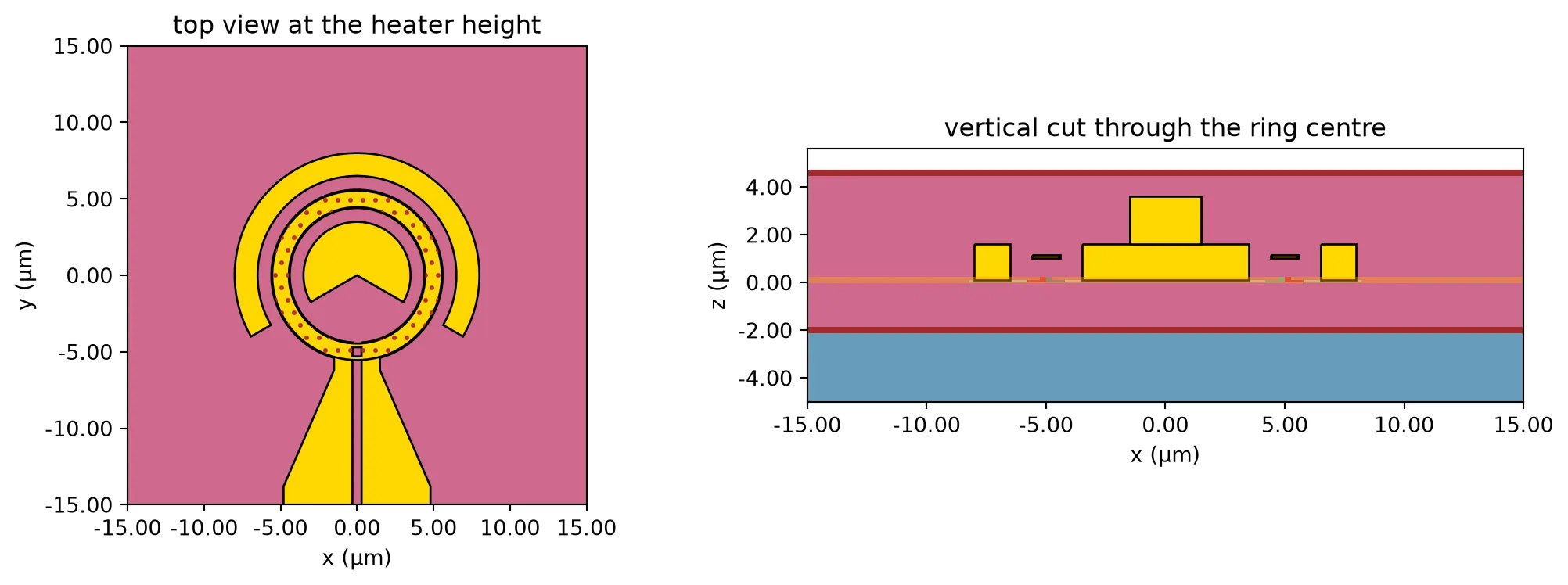

The simulation switches on 1 mW in the heater at time zero and records the temperature of the ring core.

# Run the transient simulation
data_t = web.Job(simulation=sim_t, task_name="oio_heat_transient", verbose=False).run(
    path="heat_transient.hdf5"
)

# Read the temperature history at one point on the ring core, away from the slot
probe = data_t["wg_plane"].temperature.interp(x=r_target, y=0.0, z=z_wg)
t_us = np.asarray(probe.coords["t"].values) * 1e6  # Time axis (us)

# Normalise the temperature rise to its final value
rise = np.asarray(probe.values, float).squeeze() - 300.0
rise /= rise[-1]

# Take the time to reach 1 - 1/e of the final value as the time constant
tau_us = float(np.interp(1 - np.exp(-1), rise, t_us))
f_thermal = 1 / (2 * np.pi * tau_us * 1e-6)  # Corner frequency of the heater (Hz)

fig, ax = plt.subplots(figsize=(6.5, 3.2), tight_layout=True)
ax.plot(t_us, rise, "-o", ms=2.5, lw=1)
ax.axvline(tau_us, color="gray", ls="--", lw=1)
ax.axhline(1 - np.exp(-1), color="gray", ls=":", lw=1)
ax.set(
    xlabel="time (us)",
    ylabel="ring temperature rise, normalised",
    title=f"heater step response, time constant {tau_us:.1f} us",
)
ax.grid(alpha=0.3)
plt.show()

print(f"time constant            {tau_us:.1f} us")
print(f"thermal corner frequency {f_thermal*1e-3:.1f} kHz")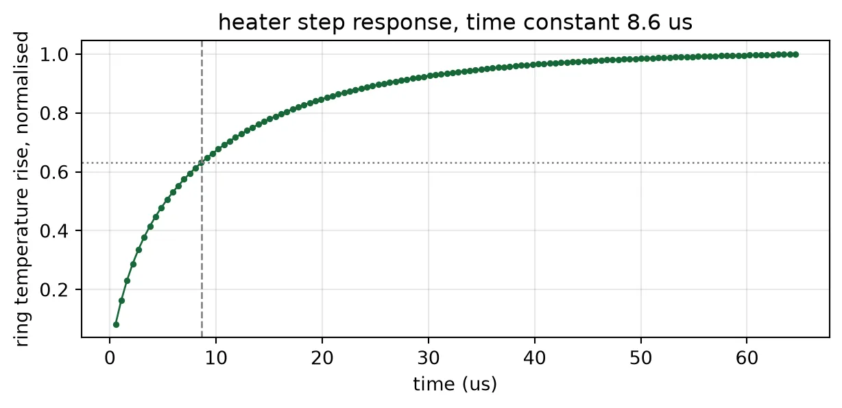

time constant            8.6 us
thermal corner frequency 18.4 kHz

The ring temperature reaches 63% of its final value after about 9 us, so the heater follows changes up to about 18 kHz. This has two consequences for the loops on this page:

• Dither frequencies of a few kilohertz reach the ring with little reduction in amplitude.
• The feedback loops run at a few tens of hertz, because a lock-in amplifier must average over many dither periods. At these frequencies the heater responds instantly, so the loop simulations later on this page treat the heater as an instantaneous gain.

Locking the drop filter

The drop filter from Component Library consists of two coupled racetrack resonators, designed for a flat passband [4]. Each racetrack has its own heater, and Chip Layout connects all four heater terminals to separate bond pads. The layout below shows the two heaters, one above each racetrack.

# Show the filter cell, with one heater on each racetrack
viewer(second_order)

Why each filter needs two loops

Each heater shifts the resonance of its own racetrack. With two heaters, the filter can be tuned in two independent ways:

• Common-mode tuning: both resonances shift in the same direction. This moves the passband without changing its shape.
• Differential tuning: the two resonances shift in opposite directions. This changes the separation between them.

Differential tuning is needed because fabrication does not produce identical racetracks. The ring-to-ring spread measured in Wavelength Plan and Thermal Budget, one standard deviation $\sigma$, applies to each racetrack independently, so the two racetracks of one filter typically differ by $\sqrt{2}\,\sigma$.

The filter model has a separate temperature for each racetrack. The cell below separates the two resonances by increasing amounts while keeping their average fixed, and reads the response at the centre of the passband, where the channel is.

# Take the parameters of the filter's model, which has one temperature per racetrack
pair_kwargs = dict(second_order.models["dual ring"].parametric_kwargs)

def detuned_filter(shift_a, shift_b):
    """Filter with its two racetrack resonances shifted by shift_a and shift_b (GHz).

    A positive shift moves a resonance up in frequency, which means a cooler ring.
    """
    # Rebuild the model with its own temperature on each racetrack
    model = pf.DualRingModel(
        **{
            **pair_kwargs,
            "temperature1": t_ref - shift_a / ghz_per_k_strip,
            "temperature2": t_ref - shift_b / ghz_per_k_strip,
        }
    )
    return model.black_box_component(port_spec="TE_1550_500")

bit_rate = 100e9  # Line rate per channel (bit/s)

# Frequency offsets from the design frequency (Hz)
offsets = np.arange(-500e9, 500e9, 0.5e9)

# Separate the two resonances by increasing multiples of the measured spread
aparts = [0.0, sigma_ring, np.sqrt(2) * sigma_ring, 2 * np.sqrt(2) * sigma_ring]

print(
    f"{'apart GHz':>10s} {'3 dB width GHz':>15s} {'ripple dB':>10s} "
    f"{'loss dB':>8s} {'rejection dB':>13s}"
)
fig, ax = plt.subplots(figsize=(6.5, 3.8), tight_layout=True)
for apart in aparts:
    # Shift the two racetracks in opposite directions, keeping their average fixed
    cell = detuned_filter(apart / 2, -apart / 2)

    # Read the drop-port transmission
    drop = (
        np.abs(cell.s_matrix(f0 + offsets, show_progress=False)["in@0", "drop@0"]) ** 2
    )

    # Find the band edges at half the highest point, and the centre between them
    band = offsets[drop >= 0.5 * drop.max()]
    centre = 0.5 * (band.min() + band.max())

    # Read the level at the centre and at the worse of the two neighbouring channels
    here = np.interp(centre, offsets, drop)
    neighbour = max(
        np.interp(centre + s * channel_grid, offsets, drop) for s in (-1, 1)
    )

    # Measure the ripple over the middle of the band, where the signal is
    signal = np.abs(offsets - centre) <= bit_rate / 2
    ripple = 10 * np.log10(drop[signal].max() / drop[signal].min())

    print(
        f"{apart:10.1f} {(band.max()-band.min())*1e-9:15.1f} {ripple:10.2f} "
        f"{-10*np.log10(here):8.2f} {10*np.log10(neighbour/here):13.1f}"
    )
    ax.plot(offsets * 1e-9, 10 * np.log10(drop), label=f"{apart:.0f} GHz apart")

ax.axvspan(
    -bit_rate * 1e-9 / 2,
    bit_rate * 1e-9 / 2,
    color="tab:orange",
    alpha=0.15,
    label="100 Gb/s signal",
)
for s in (-1, 1):
    ax.axvline(s * channel_grid * 1e-9, ls="--", c="0.5", lw=1)
ax.set(
    xlabel="offset from the design frequency (GHz)",
    ylabel="drop port (dB)",
    xlim=(-400, 400),
    ylim=(-30, 2),
)
ax.grid(alpha=0.3)
ax.legend(fontsize=8)
plt.show()

 apart GHz  3 dB width GHz  ripple dB  loss dB  rejection dB
       0.0           142.0       0.63     0.26         -18.7
      45.6           155.0       0.34     1.22         -17.7
      64.5           166.0       0.54     2.09         -16.7
     129.0           218.0       1.31     6.00         -12.1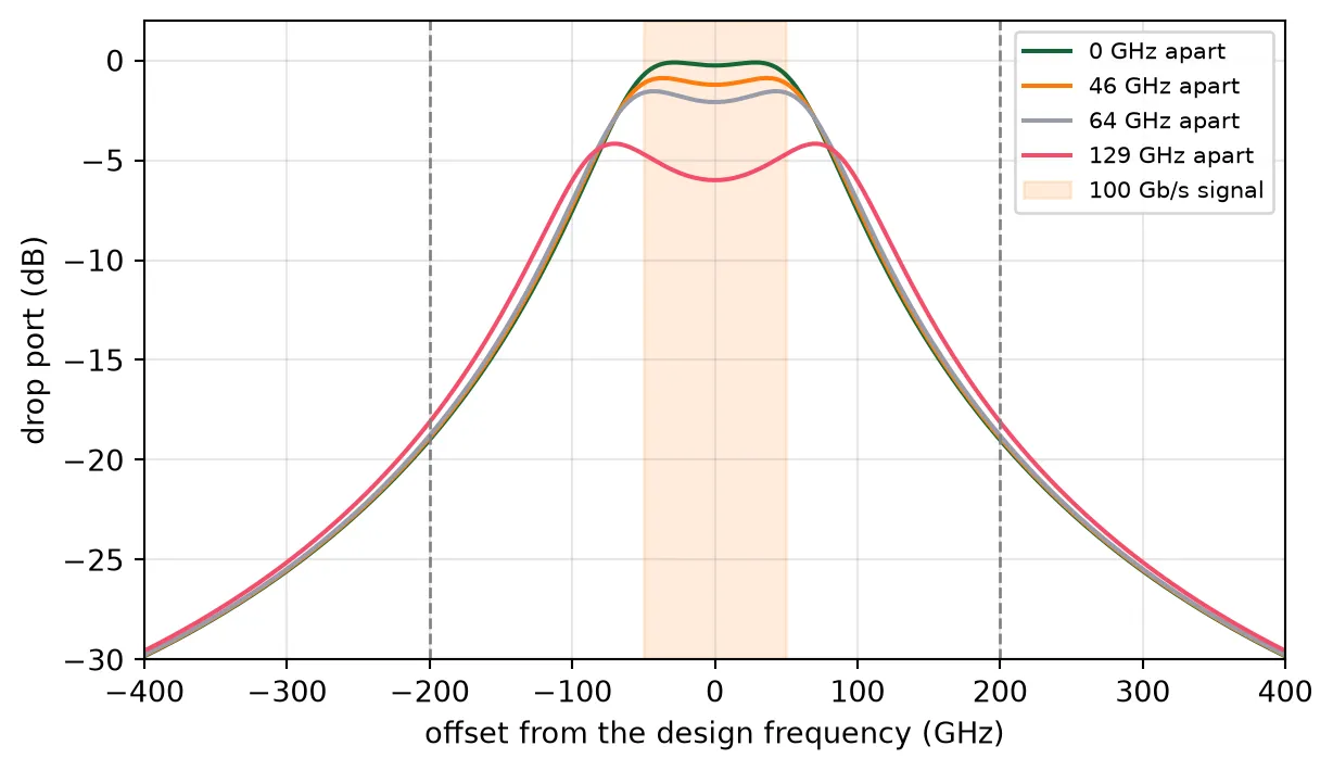

Separating the resonances changes the passband shape only slightly: the ripple across the 100 GHz occupied by the signal stays near 1 dB. The main effect is a loss. Light has to pass through two resonances that no longer coincide, so the transmission at the passband centre falls. For the typical mismatch of $\sqrt{2}\,\sigma$, about 65 GHz, the loss is about 2 dB; for twice that mismatch it is 6 dB.

Common-mode tuning cannot recover this loss, because it does not change the separation of the two resonances. Only differential tuning can, and that requires a loop on each of the two heaters.

Error signal from a dither

The error signal for each filter heater is obtained in four steps.

1. A small sinusoid at frequency $f_d$ is added to the heater power. It shifts that racetrack’s resonance by $\delta \sin(2 \pi f_d t)$, where $\delta$ is the peak resonance shift caused by the dither.

2. As the resonance moves, the detected power changes with it. For a small $\delta$, a first-order Taylor expansion of the mean detected power $\bar{P}$ in the resonance position $\Delta$ gives

   $$P(t) \approx \bar{P}(\Delta) + \delta \, \frac{d \bar{P}}{d \Delta} \, \sin(2 \pi f_d t) .$$

3. A lock-in amplifier multiplies the photodiode signal by $\sin(2 \pi f_d t)$ and averages over many periods. Only the term at $f_d$ survives the average, and the output is

   $$H_1 = \delta \, \frac{d \bar{P}}{d \Delta} .$$

4. $H_1$ is proportional to the slope of $\bar{P}$. It is zero at a maximum of $\bar{P}$ and has opposite signs on the two sides of it. The loop adjusts the heater power until $H_1 = 0$.

The mean detected power $\bar{P}$ is the photocurrent averaged over many bits. It equals the drop transmission $T$ weighted by the power spectrum $S$ of the signal:

$$\bar{P}(\Delta) = \frac{\int S(f) \, T(f - \Delta) \, df}{\int S(f) \, df} .$$

For non-return-to-zero (NRZ) data at bit rate $B$, $S(f) \propto \mathrm{sinc}^2(f/B)$. An unmodulated laser, a continuous-wave (CW) probe, corresponds to $B \to 0$, where $\bar{P}$ is simply $T$ at the carrier frequency.

The loop holds the passband centred on the carrier only if $\bar{P}$ has a maximum there. The table below checks this. For common-mode tuning it gives the second derivative of $\bar{P}$ with respect to the shift of both resonances; for differential tuning, the second derivative with respect to their separation. Both are evaluated with the passband centred on the carrier. A negative value means a maximum, where the loop is stable.

# Frequency grid for the average over the signal spectrum (Hz)
spread = np.arange(-400e9, 400.1e9, 2e9)

def mean_drop(shift_a, shift_b, rate):
    """Mean detected drop power for NRZ data at a bit rate, or for a CW probe if rate is 0."""
    # Read the drop-port transmission of the detuned filter
    cell = detuned_filter(shift_a, shift_b)
    drop = (
        np.abs(cell.s_matrix(f0 + spread, show_progress=False)["in@0", "drop@0"]) ** 2
    )

    # Return the transmission at the carrier for a CW probe
    if rate == 0:
        return float(np.interp(0.0, spread, drop))

    # Weight the transmission by the NRZ power spectrum
    weight = np.sinc(spread / rate) ** 2
    return float(np.sum(weight * drop) / np.sum(weight))

step = 10.0  # Finite-difference step for the second derivative (GHz)

print(f"{'bit rate':>10s} {'common mode':>12s} {'differential':>13s}   (per 100 GHz^2)")
for rate in (0, 25e9, 50e9, 100e9, 200e9):
    # Take the second difference for each tuning direction, around the centred passband
    centre = mean_drop(0, 0, rate)
    common = mean_drop(step, step, rate) - 2 * centre + mean_drop(-step, -step, rate)
    diff = (
        mean_drop(step / 2, -step / 2, rate)
        - 2 * centre
        + mean_drop(-step / 2, step / 2, rate)
    )
    label = "CW" if rate == 0 else f"{rate*1e-9:.0f} Gb/s"
    print(f"{label:>10s} {common/step**2*1e4:+12.3f} {diff/step**2*1e4:+13.3f}")

# Compare the mean detected power under common-mode tuning, for CW and for data
shifts = np.arange(-120.0, 120.1, 2.0)
fig, ax = plt.subplots(figsize=(6.5, 3.4), tight_layout=True)
for rate, label in ((0, "CW probe"), (bit_rate, "100 Gb/s NRZ")):
    # Read the mean detected power across the common-mode shifts
    p = np.array([mean_drop(s, s, rate) for s in shifts])
    ax.plot(shifts, p / p.max(), label=label)
ax.set(
    xlabel="passband offset from the carrier (GHz)",
    ylabel="mean detected power, normalised",
)
ax.grid(alpha=0.3)
ax.legend()
plt.show()

  bit rate  common mode  differential   (per 100 GHz^2)
        CW       +1.525        -2.115
   25 Gb/s       +0.775        -1.983
   50 Gb/s       -0.002        -1.854
  100 Gb/s       -1.643        -1.490
  200 Gb/s       -0.749        -0.880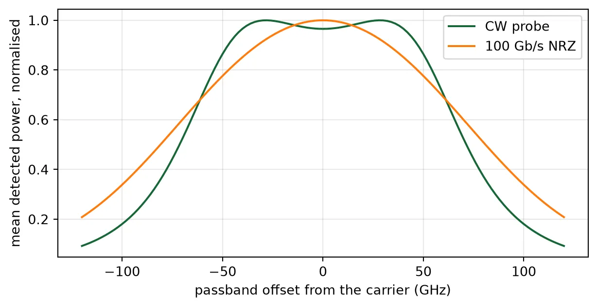

For a CW probe the second derivative in the common-mode direction is positive: the centre of the flat passband is a shallow minimum, with a maximum on each side of it. The plot shows this dip. A loop using a CW probe would therefore move the passband until the carrier sat on one of the two maxima, away from the centre.

With data, the photodiode averages the transmission over the signal spectrum, and the dip disappears. The common-mode second derivative passes through zero at 50 Gb/s, and at 100 Gb/s the passband centre is a clear maximum for both tuning directions. On this chip the data itself therefore serves as the probe: each filter loop uses the photocurrent of its own channel’s photodiode, and no separate probe laser is needed.

At 200 Gb/s the second derivative becomes smaller again, because the signal spectrum is wider than the passband.

The two error signals together

The two heaters of a filter are dithered at two different frequencies, so the lock-in amplifier gives two readings from the same photodiode: the slope of $\bar{P}$ with respect to the resonance position of each racetrack. Together they form the gradient of $\bar{P}$, and the two loops move both resonances along this gradient towards the maximum.

The map shows $\bar{P}$ for 100 Gb/s data as a function of both resonance positions, with the gradient drawn as flow lines.

grid = np.arange(-160.0, 160.1, 8.0)  # Resonance offset of each racetrack (GHz)

# Map the mean detected power over the two racetrack offsets
surface = np.array([[mean_drop(sa, sb, bit_rate) for sb in grid] for sa in grid])

# Take the gradient, which is what the two lock-in amplifiers measure
grad_a, grad_b = np.gradient(surface, grid, grid)

# Check, along each axis, how far out the gradient still points back to the centre
mid = len(grid) // 2
reach = []
for along in (grad_a[mid:, mid], grad_b[mid, mid:]):
    # A restoring gradient is negative on this side of the centre
    wrong = np.flatnonzero(along[1:] >= 0)

    # Record the last offset before the gradient changes sign
    reach.append(grid[mid:][wrong[0]] if len(wrong) else grid[-1])
capture = min(reach)  # Capture range, the smaller of the two axes (GHz)

fig, ax = plt.subplots(figsize=(5.4, 4.6), tight_layout=True)
mesh = ax.pcolormesh(
    grid,
    grid,
    10 * np.log10(surface / surface.max()),
    shading="auto",
    vmin=-15,
    vmax=0,
    cmap="viridis",
)
ax.streamplot(grid, grid, grad_b, grad_a, color="white", density=0.9, linewidth=0.7)
ax.set(
    xlabel="racetrack B offset (GHz)", ylabel="racetrack A offset (GHz)", aspect="equal"
)
fig.colorbar(mesh, ax=ax, label="mean detected power (dB)")
plt.show()

# Report the reach, which may extend past the edge of the map
edge = " (the edge of the map)" if capture >= grid[-1] else ""
print(f"the gradient points back to the centre out to {capture:.0f} GHz{edge}")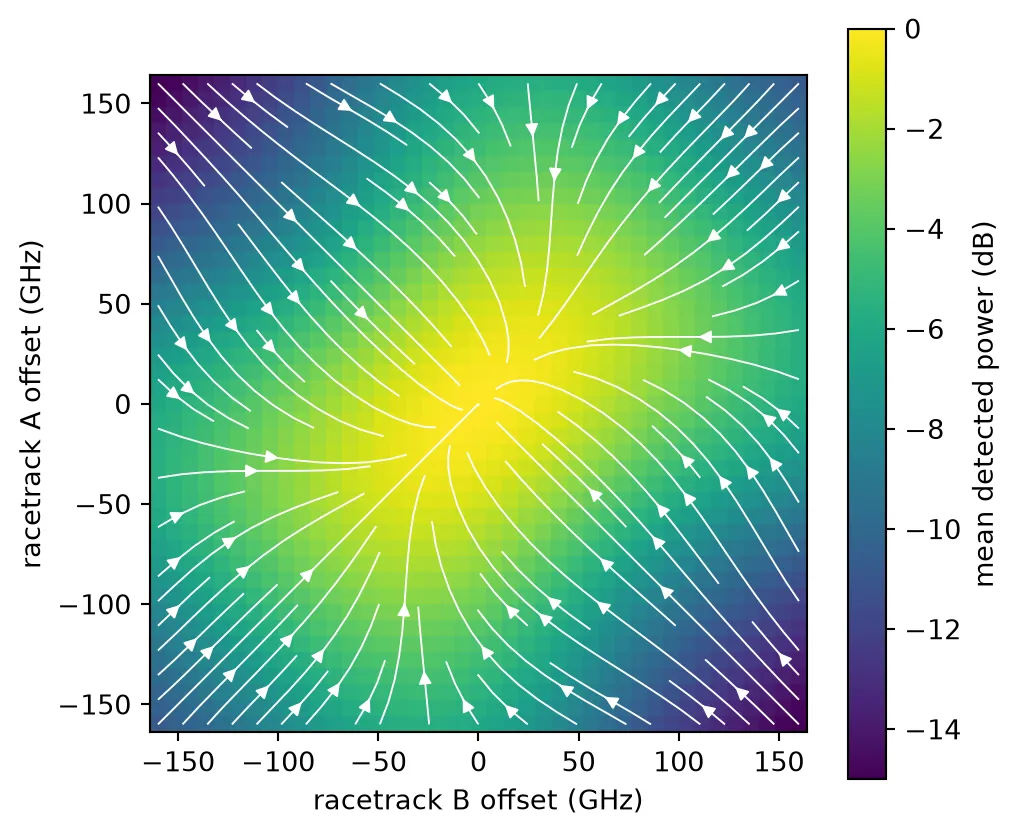

the gradient points back to the centre out to 160 GHz (the edge of the map)

All flow lines end at the centre, so the loops reach the operating point from any starting position within at least 160 GHz, well beyond the fabrication spread. The bright region is elongated along the diagonal, where both resonances move together, and narrow across it. The detected power therefore falls faster with differential mistuning than with common-mode mistuning, consistent with the loss table above.

Heat shared between the two racetracks

The thermal page measured how much heat reaches a ring 150 um away. The two racetracks of one filter are only about 10 um apart, so each heater also warms the other racetrack. This shared heating shifts both resonances in the same direction, which reduces the effect of differential tuning.

A steady HEAT simulation measures it: the heater of racetrack A is powered, and the temperature rise of both racetracks is recorded. The model is built from the layout in the same way as the transient model: the filter cell is extruded with its own technology, and the die, cladding and heat source are drawn on the FloorPlan and Heat Source layers. The heat source covers the narrow track of heater A only. The stack, materials and mesh settings are those of the thermal page.

# Read the filter's drawn geometry (um)
fk = second_order.parametric_kwargs
r_f = fk["ring_radius"]  # Racetrack bend radius
half_lc = fk["coupling_length"] / 2  # Half the straight length of each racetrack
fh_width = fk["heater_width"]  # Heater track width
fh_slot = fk["heater_slot"]  # Feed slot width

# Place the two racetrack centres, as the filter cell does
y_a = 0.0
y_b = 2 * r_f + fk["core_width"] + fk["ring_gap"]

f_inset = 0.05 * fh_width  # Gap from the heated track to the metal edges (um)
f_out = r_f + fh_width / 2 - f_inset  # Outer edge of the heated track (um)
f_in = r_f - fh_width / 2 + f_inset  # Inner edge of the heated track (um)

# Draw racetrack A's heated track: two half annuli joined by two straight strips
track = [
    pf.Circle(f_out, center=(half_lc, y_a), inner_radius=f_in, sector=(-90, 90)),
    pf.Circle(f_out, center=(-half_lc, y_a), inner_radius=f_in, sector=(90, 270)),
    pf.Rectangle((-half_lc, y_a - f_out), (half_lc, y_a - f_in)),
    pf.Rectangle((-half_lc, y_a + f_in), (half_lc, y_a + f_out)),
]

# Remove the feed slot, which crosses the lower straight
heated_a = pf.boolean(
    track, [pf.Rectangle(center=(0, y_a - r_f), size=(fh_slot, 2 * fh_width))], "-"
)

# Calculate the heated volume from the drawn track
track_volume = sum(shape.area() for shape in heated_a) * h_heater

# Draw the floor plan and the heated track, as for the modulator
(fx0, fy0), (fx1, fy1) = second_order.bounds()
x0, x1 = fx0 - lateral_pad, fx1 + lateral_pad
y0, y1 = fy0 - lateral_pad, fy1 + lateral_pad
fil_floor = pf.Component("FILTER_FLOOR_PLAN", technology=heat_tech)
fil_floor.add("FloorPlan", pf.Rectangle((x0, y0), (x1, y1)))
fil_source = pf.Component("FILTER_HEAT_SOURCE", technology=heat_tech)
fil_source.add("Heat Source", *heated_a)

# Extrude the floor plan, the filter and the heated track, as for the modulator
floor = [s.to_tidy3d() for s in fil_floor.extrude(classification="electrical")]
floor = [s.updated_copy(name="wafer") if s.medium.name == "Si" else s for s in floor]
device = [s.to_tidy3d() for s in second_order.extrude(classification="electrical")]
heat_source = [
    s.to_tidy3d().updated_copy(name="heater_a")
    for s in fil_source.extrude(classification="electrical")
]

# Refine one box around both racetracks, which distance grading alone leaves coarse
refinement = td.GridRefinementRegion(
    center=(0, 0.5 * (y_a + y_b), 0.5 * (z_heater - h_box)),
    size=(4 * r_f + 2 * half_lc, 4 * r_f + y_b, 2 * h_box + z_heater + 4),
    dl_internal=0.6,
    transition_thickness=1.5 * r_f,
)

# Build the steady model from the extruded layout
sim_f = td.HeatChargeSimulation(
    center=((x0 + x1) / 2, (y0 + y1) / 2, (zb + zt) / 2),
    size=(x1 - x0, y1 - y0, zt - zb),
    structures=floor + device + heat_source,
    medium=air["electrical"],
    # Drive racetrack A only, as a volumetric rate over its track
    sources=[td.HeatSource(structures=["heater_a"], rate=p_probe / track_volume)],
    boundary_spec=[
        td.HeatBoundarySpec(
            placement=td.MediumMediumInterface(mediums=["Air", "SiO2"]),
            condition=td.ConvectionBC(ambient_temperature=300, transfer_coeff=10e-12),
        ),
        # Sink the heat at the back of the die, on the air to silicon interface
        td.HeatBoundarySpec(
            placement=td.MediumMediumInterface(mediums=["Air", "Si"]),
            condition=td.TemperatureBC(temperature=300),
        ),
    ],
    monitors=[
        td.TemperatureMonitor(
            size=(td.inf, td.inf, 0),
            center=(0, 0, z_wg),
            name="wg_plane",
            unstructured=True,
        )
    ],
    grid_spec=td.DistanceUnstructuredGrid(
        dl_interface=h_heater / 2,
        dl_bulk=25.0,
        distance_interface=h_heater,
        distance_bulk=h_box + 2,
        # Leave the substrate interior coarse, since nothing reads it
        non_refined_structures=["wafer"],
        mesh_refinements=[refinement],
        # Allow elements far smaller than the domain, which is otherwise the floor
        relative_min_dl=0.5 * (h_heater / 2) / max(x1 - x0, y1 - y0, zt - zb),
    ),
)

The plots show the model at the heater height, with heater A’s heated track inside the drawn heater of racetrack A, at the waveguide height, with the two racetrack cores, and in a vertical cut across the straight sections of both racetracks, away from the feed slots.

# Set the plotted region around the filter (um)
fil_x = (-half_lc - 2 * r_f, half_lc + 2 * r_f)
fil_y = (y_a - 2 * r_f, y_b + 2 * r_f)

# Plot the model at the heater height, at the waveguide height, and in a vertical cut
fig, ax = plt.subplots(1, 3, figsize=(14, 4.2), tight_layout=True)
sim_f.plot(z=z_mid, ax=ax[0])
ax[0].set(xlim=fil_x, ylim=fil_y, title="top view at the heater height")
sim_f.plot(z=z_wg, ax=ax[1])
ax[1].set(xlim=fil_x, ylim=fil_y, title="top view at the waveguide height")
# Cut across the straight sections, away from the feed slots at x = 0
sim_f.plot(x=half_lc / 2, ax=ax[2])
ax[2].set(
    xlim=fil_y, ylim=(-1, clad_top - 2), title="vertical cut across both racetracks"
)
plt.show()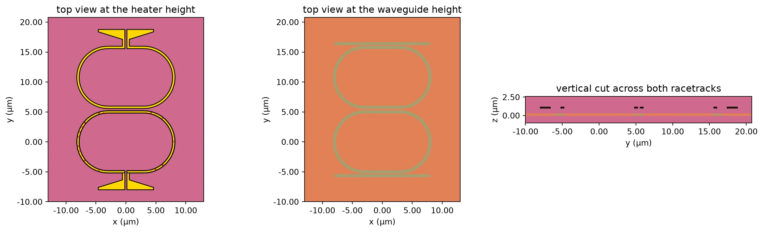

# Run the steady simulation
data_f = web.Job(simulation=sim_f, task_name="oio_heat_filter_pair", verbose=False).run(
    path="heat_filter_pair.hdf5"
)

# Read the waveguide-plane temperature and convert it to a rise above ambient
t_plane = data_f["wg_plane"].temperature
pts = np.asarray(t_plane.points.values)
vals = np.asarray(t_plane.values).reshape(-1) - 300.0

# Average the rise over each racetrack's core, a stadium of radius r_f
rises = []
for yc in (y_a, y_b):
    # Measure each point's distance from the racetrack's straight centre line
    along = np.clip(np.abs(pts[:, 0]) - half_lc, 0, None)
    dist = np.hypot(along, pts[:, 1] - yc)

    # Average the points within a quarter micron of the core centre line
    rises.append(vals[np.abs(dist - r_f) < 0.25].mean())

# Temperature rise on the driven racetrack and on its neighbour (K)
rise_a, rise_b = rises

# Fraction of the driven racetrack's rise that reaches the other one
intra = rise_b / rise_a

print(f"racetrack A, driven      {rise_a/(p_probe*1e3):.2f} K/mW")
print(f"racetrack B, neighbour   {rise_b/(p_probe*1e3):.2f} K/mW")
print(f"shared fraction          {intra:.2f}")

racetrack A, driven      4.62 K/mW
racetrack B, neighbour   1.47 K/mW
shared fraction          0.32

About a third of the temperature rise of the heated racetrack reaches the other one. The driven racetrack rises by 4.6 K per milliwatt, more than the 3.5 K per milliwatt of the modulator, for two geometric reasons: the filter’s heater is narrower, and the filter has no silicon slab, which in the modulator spreads heat sideways. The loop simulation below uses both measured values for the filters.

The shared heating reduces the effect of differential tuning. When the two heater powers are changed by $+p$ and $-p$, the separation of the two resonances changes by $(1 - c)$ times what it would without shared heating, where $c$ is the shared fraction. With $c$ about 0.3, the differential loop needs about 1.5 times more heater power for the same correction, which the loops below include.

Locking the modulator

The operating point

A ring modulator changes the transmitted intensity through the slope of its transmission spectrum, so it is operated on the side of the resonance where this slope is largest. Link Simulation places the laser $\mathrm{FWHM}/(2\sqrt{3})$ below the resonance, where FWHM is the full width at half maximum. At this point the slope is largest, so the second derivative of the transmission is zero. A point where the second derivative of a curve is zero and changes sign is called an inflection point.

The cell below computes the transmission from the modulator’s model, without drive voltage and at the full drive voltage. The drive moves the resonance, which is how the modulator encodes data.

# Take the parameters of the modulator's model, which accepts a drive voltage
ring_kwargs = dict(mrm.models["ring"].parametric_kwargs)

v_drive = 3.0  # Modulator peak-to-peak drive voltage (V)

# Probe frequency offset from the resonance at 0 V (Hz), and the same in GHz
scan = np.arange(-300e9, 300.1e9, 0.25e9)
x = scan * 1e-9

# Calculate the transmission at 0 V and at the full drive
lines = []
for v in (0.0, v_drive):
    # Build the ring at this voltage and read its through-port transmission
    ring = pf.RingModel(**{**ring_kwargs, "voltage": v}).black_box_component(
        port_spec="Rib_TE_1550_500"
    )
    lines.append(
        np.abs(ring.s_matrix(f0 + scan, show_progress=False)["P0@0", "P1@0"]) ** 2
    )
t_off, t_on = lines  # Transmission at 0 V and at the full drive

# Find the linewidth at 0 V, and the operating point below the resonance
deepest = t_off.min()
inside = x[t_off <= deepest + 0.5 * (t_off.max() - deepest)]
fwhm_mod = inside.max() - inside.min()

# Operating point, FWHM/(2 sqrt 3) below the resonance (GHz)
bias = -fwhm_mod / (2 * np.sqrt(3))

fig, ax = plt.subplots(figsize=(6.5, 3.4), tight_layout=True)
ax.plot(x, t_off, label="0 V")
ax.plot(x, t_on, label=f"{v_drive:.0f} V")
ax.axvline(bias, color="#c8385a", ls="--", lw=1, label="operating point")
ax.set(
    xlabel="laser offset from the 0 V resonance (GHz)",
    ylabel="transmission",
    xlim=(-150, 100),
)
ax.grid(alpha=0.3)
ax.legend()
plt.show()

print(f"linewidth (FWHM)            {fwhm_mod:.1f} GHz")
print(f"operating point             {bias:.1f} GHz")
print(f"resonance shift at {v_drive:.0f} V      {x[np.argmin(t_on)]:+.1f} GHz")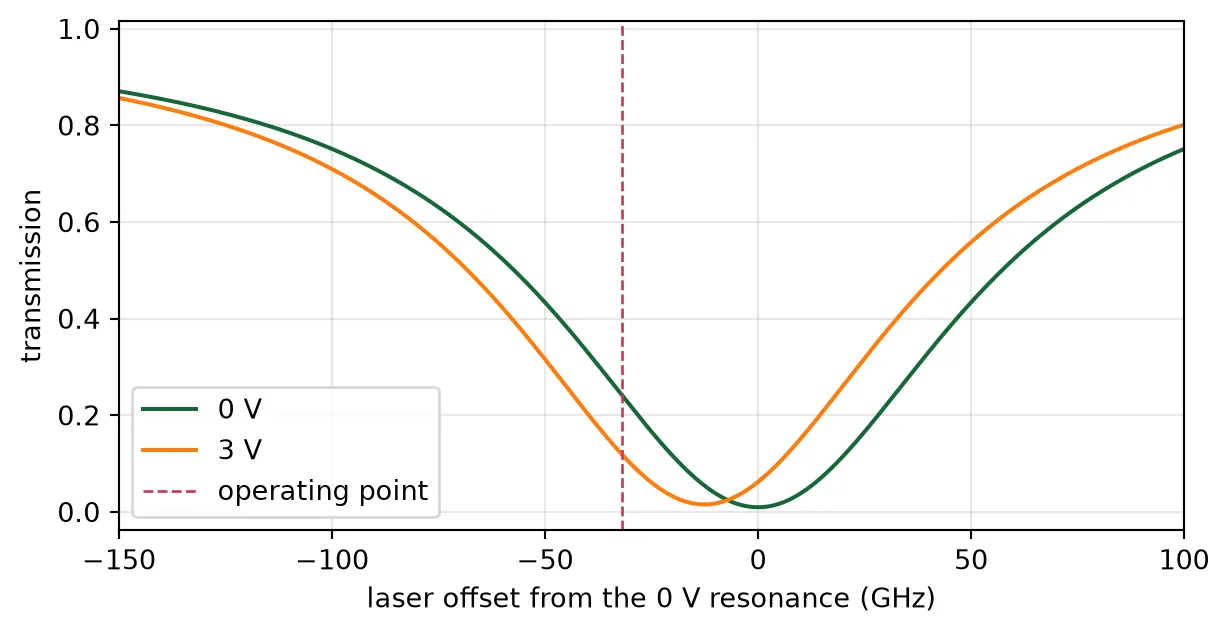

linewidth (FWHM)            111.0 GHz
operating point             -32.0 GHz
resonance shift at 3 V      -12.5 GHz

Why the filter’s error signal does not work here

Two simpler methods fail for the modulator on this chip.

• The first-harmonic signal, $H_1$, used for the filter is proportional to the slope of the transmission. A loop that drives $H_1$ to zero moves the laser to the point where the slope is zero, which is the transmission minimum at the resonance itself. Because the slope is zero there, the drive voltage produces almost no change in the transmitted intensity.
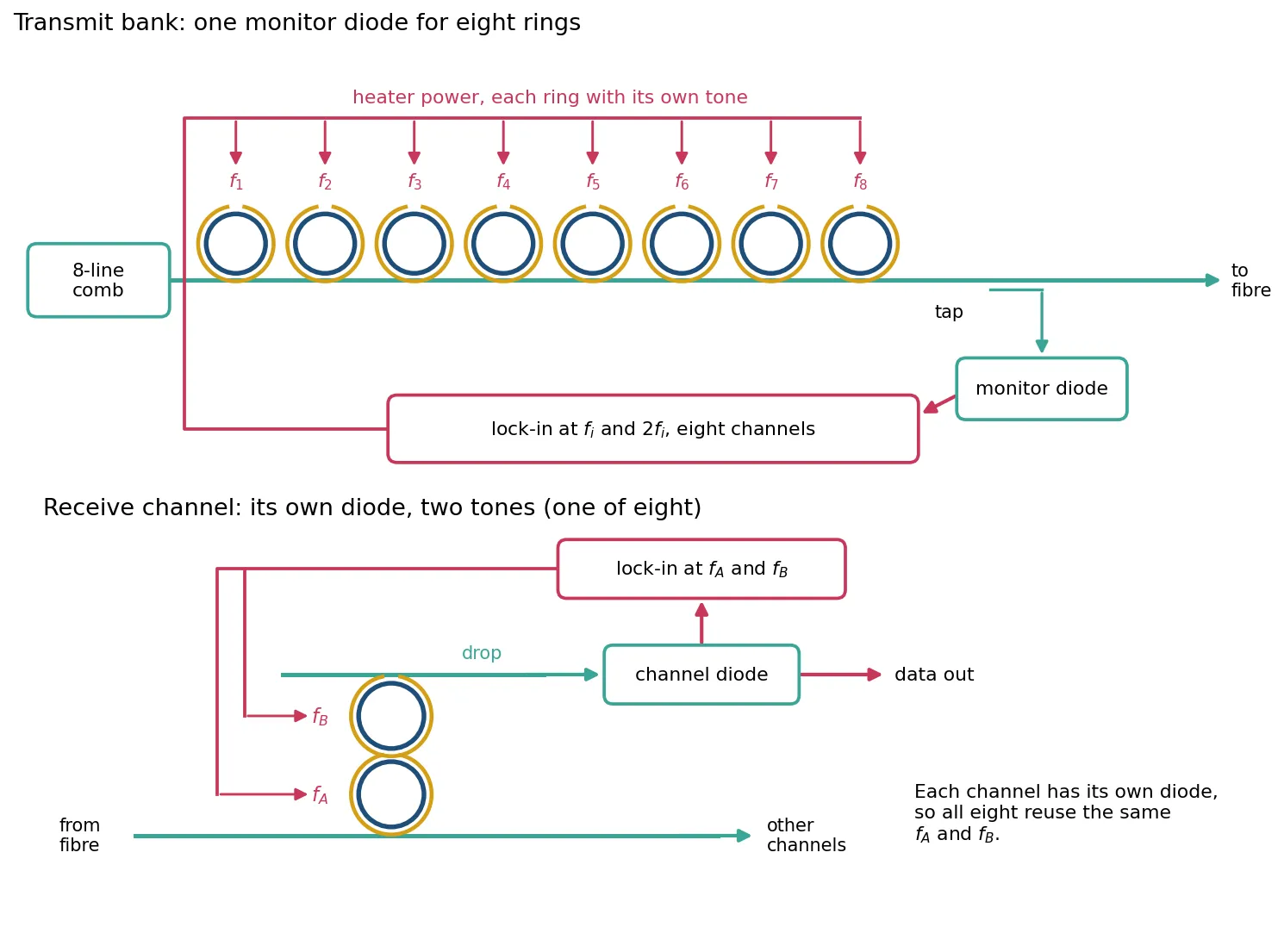
• Holding the photodiode current at a fixed value [3] works for a single ring with its own photodiode. On this chip the modulators share one photodiode behind a tap at the output of the transmit bank (see Chip Layout), and this photodiode receives all eight carriers. Most of its current comes from the other seven channels, and a change in laser power or coupling loss changes the current even when the ring has not moved. A cell below quantifies this.

Error signal from the second harmonic

The modulator heater is dithered in the same way as the filter heaters: a small sinusoid at frequency $f_d$ is added to the heater power. The dither size is given by the peak resonance shift $\delta$ it causes. A dither of $\delta = 5$ GHz corresponds to 0.15 mW of heater power.

Expanding the transmission $T$ to second order in $\delta$, with $x$ the laser offset from the resonance and $\omega = 2 \pi f_d$:

$$T(x + \delta \sin \omega t) \approx T(x) + \delta \, T'(x) \sin \omega t + \frac{\delta^2}{2} \, T''(x) \sin^2 \omega t .$$

Since $\sin^2 \omega t = (1 - \cos 2 \omega t)/2$, the photodiode signal contains a component at twice the dither frequency, $-(\delta^2/4) \, T''(x) \cos 2 \omega t$. A lock-in amplifier referenced to $2 f_d$ measures

$$H_2 = -\frac{\delta^2}{4} \, T''(x) .$$

$H_2$ is zero at the inflection point, which is the operating point, and changes sign across it, so it is a suitable error signal. The position of its zero does not depend on how much light reaches the photodiode: a change in optical power scales $H_2$ but does not move its zero. Each modulator heater is dithered at a different frequency, so the lock-in amplifier at twice that frequency measures only that ring, although all eight carriers reach the same photodiode. The figure below shows this arrangement for both banks.

The cell below computes $H_1$ and $H_2$ as functions of the laser offset, for a 5 GHz dither.

n_phase = 64  # Samples per dither period
phase = 2 * np.pi * (np.arange(n_phase) + 0.5) / n_phase  # Dither phase over one period

def harmonics(line, x_laser, shift):
    """Lock-in outputs at the dither frequency and at twice it.

    line is a transmission against laser offset, x_laser the mean laser offset (GHz),
    and shift the resonance shift over one dither period (GHz).
    """
    # Sample the transmission over one dither period
    p = np.interp(x_laser + shift, x, line)
    return 2 * np.mean(p * np.sin(phase)), 2 * np.mean(p * np.cos(2 * phase))

def null(line, shift, lo=-90.0, hi=-1.0):
    """Laser offset below the resonance where the second-harmonic output is zero."""
    trial = np.arange(lo, hi, 0.05)  # Laser offsets to search (GHz)
    h2 = np.array([harmonics(line, xl, shift)[1] for xl in trial])

    # Locate the sign change and interpolate across it
    k = np.flatnonzero(np.diff(np.sign(h2)))[0]
    return trial[k] - h2[k] * (trial[k + 1] - trial[k]) / (h2[k + 1] - h2[k])

dither = 5.0  # Peak resonance shift caused by the dither (GHz)

# Calculate both lock-in outputs across the lower side of the resonance
x_read = np.arange(-120.0, -1.0, 0.5)
readings = np.array([harmonics(t_off, xl, dither * np.sin(phase)) for xl in x_read])

# Find the zero of the second-harmonic output
null_cw = null(t_off, dither * np.sin(phase))

fig, ax = plt.subplots(3, 1, figsize=(6.5, 6.4), sharex=True, tight_layout=True)
ax[0].plot(x, t_off)
ax[0].set(ylabel="transmission")
ax[1].plot(x_read, readings[:, 0])
ax[1].set(ylabel="$H_1$")
ax[2].plot(x_read, readings[:, 1])
ax[2].set(
    ylabel="$H_2$", xlabel="laser offset from the resonance (GHz)", xlim=(-120, 20)
)
for a in ax:
    a.axvline(bias, color="#c8385a", ls="--", lw=1)
    a.grid(alpha=0.3)
plt.show()

print(f"operating point             {bias:.1f} GHz")
print(f"zero of H2, {dither:.0f} GHz dither    {null_cw:.1f} GHz")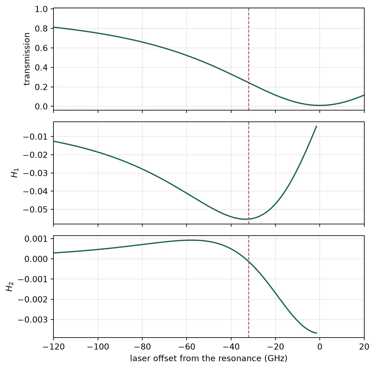

operating point             -32.0 GHz
zero of H2, 5 GHz dither    -33.4 GHz

$H_2$ crosses zero at the operating point, marked by the dashed line, where $H_1$ is largest. The zero lies 1.4 GHz from $\mathrm{FWHM}/(2\sqrt{3})$, because the dither averages the transmission over a range of a few gigahertz. The table below shows this offset growing with the dither amplitude, and compares the second-harmonic lock with a lock that holds the photodiode current at a fixed value.

print(f"{'dither GHz':>11s} {'zero of H2 GHz':>15s} {'offset GHz':>11s}")
for amp in (5.0, 10.0, 20.0, 30.0):
    # Find the zero of the second-harmonic output for this dither amplitude
    z = null(t_off, amp * np.sin(phase))
    print(f"{amp:11.0f} {z:15.1f} {z - bias:11.1f}")

# Hold the transmission a fixed-current lock would hold, then reduce the light by 1 dB
target = np.interp(bias, x, t_off)
lower = (x > -150) & (x < 0)  # The side of the resonance below the carrier

# Find where the reduced reading equals the held value
held = np.interp(target * 10**0.1, t_off[lower][::-1], x[lower][::-1])

print()
print(f"a fixed-current lock moves by {held - bias:+.1f} GHz for 1 dB less light")
print("the zero of H2 does not move, because the light level scales all of H2")

 dither GHz  zero of H2 GHz  offset GHz
          5           -33.4        -1.4
         10           -33.8        -1.8
         20           -35.3        -3.2
         30           -37.6        -5.5

a fixed-current lock moves by -5.7 GHz for 1 dB less light
the zero of H2 does not move, because the light level scales all of H2

With a 5 GHz dither the zero of $H_2$ is 1.4 GHz from $\mathrm{FWHM}/(2\sqrt{3})$, about 1% of the linewidth. A loop that holds the photodiode current at a fixed value moves by about 6 GHz when the received light changes by 1 dB. The zero of $H_2$ does not move.

Locking while the modulator transmits data

During operation the modulator transmits data. The drive voltage switches the resonance between the two positions shown in the first plot of this section, one for each bit value. The lock-in amplifier averages over many bits, so with equal numbers of ones and zeros it measures $H_2$ of the average of the two transmission curves. The zero of $H_2$ is then the inflection point of this average curve, not of the 0 V curve.

The cell below finds this zero. It also computes the modulation amplitude, the difference between the transmissions of the two drive states at a given laser position, and finds where it is largest.

# Average the two drive states, as the lock-in amplifier does over many bits
t_data = 0.5 * (t_off + t_on)

# Find the zero of H2 with data
null_data = null(t_data, dither * np.sin(phase))

# Calculate the modulation amplitude, and find where it is largest below the resonance
swing = np.abs(t_off - t_on)
below = x < 0
x_best = x[below][np.argmax(swing[below])]

print(
    f"zero of H2 without data          {null_cw:6.1f} GHz, "
    f"modulation amplitude {np.interp(null_cw, x, swing):.3f}"
)
print(
    f"zero of H2 with data             {null_data:6.1f} GHz, "
    f"modulation amplitude {np.interp(null_data, x, swing):.3f}"
)
print(
    f"largest modulation amplitude at  {x_best:6.1f} GHz, "
    f"modulation amplitude {swing[below].max():.3f}"
)

fig, ax = plt.subplots(figsize=(6.5, 3.4), tight_layout=True)
ax.plot(x, swing)
ax.axvline(null_cw, color="0.5", ls="--", lw=1, label="zero of $H_2$ without data")
ax.axvline(null_data, color="#c8385a", ls="--", lw=1, label="zero of $H_2$ with data")
ax.set(
    xlabel="laser offset from the 0 V resonance (GHz)",
    ylabel="modulation amplitude",
    xlim=(-120, 20),
)
ax.grid(alpha=0.3)
ax.legend()
plt.show()

zero of H2 without data           -33.4 GHz, modulation amplitude 0.125
zero of H2 with data              -40.6 GHz, modulation amplitude 0.127
largest modulation amplitude at   -38.5 GHz, modulation amplitude 0.127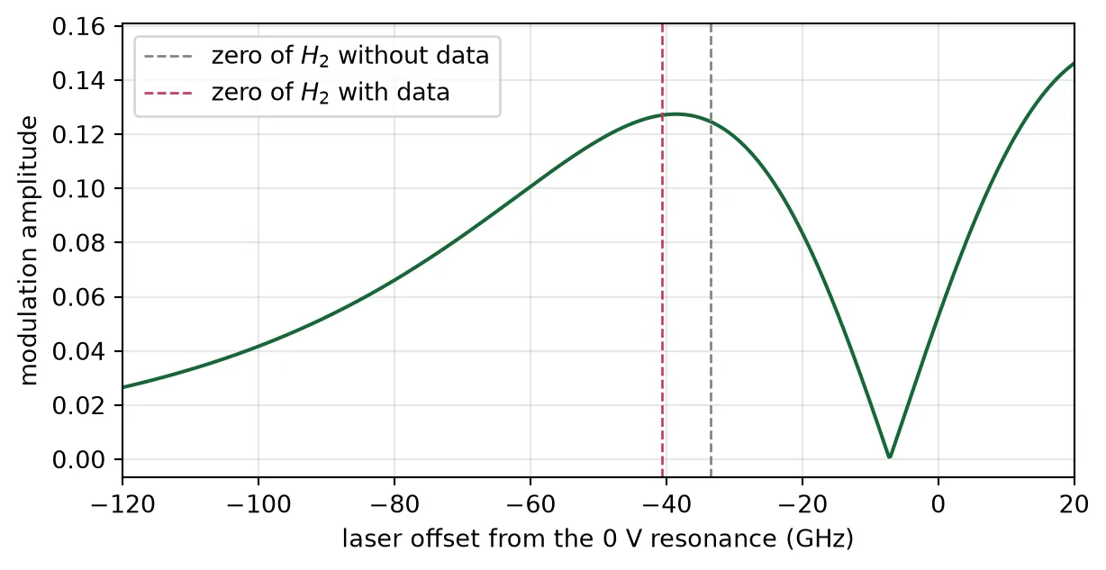

With data, the zero of $H_2$ lies 7 GHz further below the resonance, at −40.6 GHz. At this laser position the modulation amplitude is 0.127, the maximum of the curve. Without data the zero is at −33.4 GHz, where the modulation amplitude is 0.125. Locking while the modulator transmits data therefore places the laser at the position of largest modulation amplitude, without any calibration. All loops in the rest of this page operate with data.

Dithering the heater power rather than the heater voltage

The heater power is $P = V^2 / R$, where $V$ is the heater voltage and $R$ the heater resistance. If the dither is applied to the voltage, $V = V_0 + a \sin \omega t$, the power is

$$P = \frac{V_0^2 + a^2/2}{R} + \frac{2 V_0 a}{R} \sin \omega t - \frac{a^2}{2R} \cos 2 \omega t .$$

The last term is a heater power modulation at twice the dither frequency. It shifts the resonance at $2 f_d$ directly, adds to the measured $H_2$, and the loop settles at a wrong position. A smaller dither does not help, because this term and the useful part of $H_2$ both scale with $a^2$. The error is larger for rings with a low heater voltage $V_0$, so it differs from ring to ring.

The cell below compares a voltage dither with a power dither of the same amplitude at $f_d$, for three heater powers from the thermal page.

# Calculate the heater resistance from the TiN conductivity and the heated track
sigma_tin = tin["electrical"].charge.conductivity  # TiN electrical conductivity (S/um)
# Take the heated track's length from its drawn area, divided by its width (um)
arc_length = sum(shape.area() for shape in heated) / (arc_r_out - arc_r_in)
r_heater = arc_length / (sigma_tin * heater_width * h_heater)  # Heater resistance (ohm)

dither_share = 0.05  # Voltage dither as a fraction of the standing voltage

print(f"heater resistance {r_heater:.0f} ohm")
print()
print(
    f"{'trim mW':>8s} {'V0':>7s} {'voltage dither':>15s} {'power dither':>13s} "
    f"{'error GHz':>10s}"
)
for p0 in (1.0, mean_mw, worst_mw):
    # Find the standing voltage for this heater power, and the voltage dither
    v0 = np.sqrt(p0 * 1e-3 * r_heater)
    a = dither_share * v0

    # Follow the resonance over one period of a voltage dither, including the square law
    by_voltage = (
        ghz_per_mw_rib * 1e3 * ((v0 + a * np.sin(phase)) ** 2 - v0**2) / r_heater
    )

    # Apply a power dither with the same amplitude at the dither frequency
    by_power = ghz_per_mw_rib * 1e3 * (2 * v0 * a / r_heater) * np.sin(phase)

    # Find the zero of H2 for each kind of dither
    z_v = null(t_data, by_voltage)
    z_p = null(t_data, by_power)
    print(f"{p0:8.2f} {v0:7.3f} {z_v:13.1f} GHz {z_p:10.1f} GHz {z_v - z_p:+10.1f}")

heater resistance 94 ohm

 trim mW      V0  voltage dither  power dither  error GHz
    1.00   0.306         -32.0 GHz      -40.5 GHz       +8.6
    4.12   0.622         -39.0 GHz      -41.4 GHz       +2.3
    8.24   0.879         -43.0 GHz      -43.9 GHz       +0.9

With a voltage dither the lock settles 8.6 GHz from the correct position at 1 mW of heater power and 0.9 GHz from it at 8.3 mW. With a power dither there is no such error: the controller sets the heater power directly and computes the voltage as $V = \sqrt{P R}$. All loops below use a power dither.

A dither lock in the time domain

The sections above use the transmission curve and the average output of the lock-in amplifier. The circuit simulation below closes one modulator loop in time, with the same structure as the dither lock in Microring Thermal Stabilization, but detecting the second harmonic. The figure shows the loop:

• The laser passes through the modulator ring to a photodiode.
• The photodiode signal is multiplied by a reference at twice the dither frequency, $\cos 2 \omega_d t$, and passed through a low-pass filter. These two blocks form the lock-in amplifier, and their output is proportional to $H_2$.
• An integrator converts this output into a heater power command.
• The command passes through a first-order low-pass filter that represents the thermal response of the heater, and the dither $\sin \omega_d t$ is added before it reaches the ring.

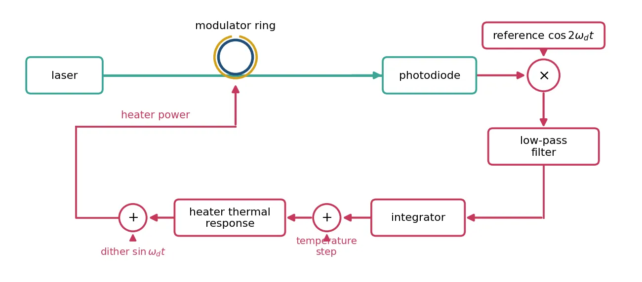
The ring is the modulator cell from Component Library, with its electrical input used as the heater input: 1 V stands for 1 mW of heater power, with the measured tuning of 33.1 GHz/mW. The input sets the heater power directly, as the previous section requires. The laser is placed so that the zero of $H_2$ for a 5 GHz dither, computed above, falls at a heater power of 2 mW. The modulator transmits no data in this simulation, so the expected operating point is the zero without data.

The time step must resolve the 0.4 ps round trip of the ring, while on the chip the loop settles in tens of milliseconds, which would take about 10¹¹ steps. The slow rates are therefore increased: the heater’s corner frequency from 18 kHz to 30 MHz, the dither from a few kilohertz to 200 MHz, and the loop bandwidth from 20 Hz to 0.33 MHz. Their order is kept. The lock-in filter is a hundredth of the dither frequency, as on the chip, so that it removes the ripple at the dither frequency and its harmonics before the integrator. The dither is added after the thermal filter, because at 200 MHz the scaled filter would attenuate it, while on the chip the kilohertz dither passes the heater with little loss.

The loop starts with the heater at 1.6 mW, 13 GHz from the operating point. At 2 us a step of 0.3 mW is added to the heater power, which represents a sudden change of the ring temperature.

# Set the time step to a quarter of the ring's round trip
tau_rt = 2 * np.pi * r_target * b["n_group"] / pf.C_0
dt = tau_rt / 4

z0 = 50.0  # Source impedance of the electrical ports (ohm)
sq = np.sqrt(z0)  # Electrical wave amplitudes are volts over sqrt(z0)
p_line = 2e-3  # Laser power per channel: +3 dBm (W)
pd_gain = 1e3  # Photodiode transimpedance (V/A)

f_th = 30e6  # Corner frequency of the heater response, scaled up (Hz)
f_d = 200e6  # Dither frequency, scaled up (Hz)
f_lp = 2e6  # Lock-in filter cutoff, a hundredth of the dither frequency (Hz)
f_c = f_lp / 6  # Loop bandwidth (Hz)

u_lock = 2.0  # Heater power at the operating point (mW)
u_start = u_lock - 0.4  # Heater power at the start (mW)
u_step = 0.3  # Heater power added by the temperature step (mW)
dither_mw = dither / ghz_per_mw_rib  # Dither amplitude as heater power (mW)

# Index change per mW of heater power, from the measured tuning
dn_heater = ghz_per_mw_rib * 1e9 * b["n_group"] / f0

# Use the modulator cell with its electrical input as the heater input, 1 V for 1 mW
heated_ring = microring_modulator(
    **{
        **mrm.parametric_kwargs,
        "dn_dv": dn_heater,
        "dn_dv2": 0.0,
        "dloss_dv": 0.0,
        "dloss_dv2": 0.0,
    }
)

# Place the laser so the zero of H2 falls at the chosen heater power
f_probe = f0 + (null_cw - ghz_per_mw_rib * u_lock) * 1e9

# Calculate the slope of the lock-in output at the zero, to set the integrator gain
v_full = pd_gain * p_line  # Detected voltage at full transmission (V)
h2_up = harmonics(t_off, null_cw + 0.5, dither * np.sin(phase))[1]
h2_down = harmonics(t_off, null_cw - 0.5, dither * np.sin(phase))[1]
de_du = v_full / 2 * (h2_up - h2_down) * ghz_per_mw_rib  # Output per mW (V/mW)
k_i = -2 * np.pi * f_c / de_du  # Integrator gain (1/s)

# Create the blocks of the loop
laser = pfa.cw_laser(power=p_line, frequency=f_probe)
monitor_pd = pfa.photodiode(responsivity=1.0, gain=pd_gain, seed=1)
mixer = pfa.multiplier(scale=sq)
lockin = pfa.filter(family="butterworth", f_cutoff=f_lp, order=2)
integrator = pfa.integrator(
    scale=k_i, start_value=u_start / sq, limits=(0.0, 10.0 / sq)
)
thermal = pfa.filter(family="rc", f_cutoff=f_th, order=1)
summer = pfa.adder()
term = pfa.electrical_termination()
dither_src = pfa.signal_source(waveform="sine", frequency=f_d, amplitude=dither_mw / sq)

# Start the reference three quarters of its period late, which makes it a cosine
reference = pfa.signal_source(
    waveform="sine", frequency=2 * f_d, amplitude=1 / sq, start=0.75 / (2 * f_d)
)

# Connect the loop, with the temperature step entering at an exposed port
loop = pf.component_from_netlist(
    {
        "name": "second-harmonic lock",
        "instances": {
            "laser": laser,
            "ring": {"component": heated_ring, "origin": (40, 0)},
            "photodiode": {"component": monitor_pd, "origin": (80, 0)},
            "mixer": {"component": mixer, "origin": (120, 0)},
            "lockin": {"component": lockin, "origin": (160, 0)},
            "controller": {"component": integrator, "origin": (200, 0)},
            "sum": {"component": summer, "origin": (240, 0)},
            "thermal": {"component": thermal, "origin": (280, 0)},
            "drive": {"component": summer, "origin": (320, 0)},
            "reference": {"component": reference, "origin": (360, 0)},
            "dither": {"component": dither_src, "origin": (400, 0)},
            "term": {"component": term, "origin": (440, 0)},
        },
        "virtual connections": [
            (("laser", "P0"), ("ring", "P0")),
            (("ring", "P1"), ("photodiode", "P0")),
            (("photodiode", "E0"), ("mixer", "E0")),
            (("reference", "E0"), ("mixer", "E1")),
            (("mixer", "E2"), ("lockin", "E0")),
            (("lockin", "E1"), ("controller", "E0")),
            (("term", "E0"), ("controller", "E1")),
            (("controller", "E2"), ("sum", "E0")),
            (("sum", "E2"), ("thermal", "E0")),
            (("thermal", "E1"), ("drive", "E0")),
            (("dither", "E0"), ("drive", "E1")),
            (("drive", "E2"), ("ring", "E0")),
        ],
        "ports": [("sum", "E1", "step")],
        "models": [(pf.CircuitModel(), "Circuit")],
    }
)

# Record the integrator output; references follow the order of the instances above
ts = loop.setup_time_stepper(
    time_step=dt,
    carrier_frequency=f_probe,
    time_stepper_kwargs={"monitors": {"command": loop.references[5]["E2"]}},
    show_progress=False,
)

t_total = 4e-6  # Simulated time (s)
t_step = 2e-6  # Time of the temperature step (s)
block = 1000  # Time steps averaged into one recorded point

# Apply the temperature step as added heater power
n_run = int(round(t_total / dt)) // block * block
t_run = np.arange(n_run) * dt
step_in = np.where(t_run >= t_step, u_step, 0.0)
out = ts.step(inputs=pf.TimeSeries({"step@0": step_in / sq}, dt), show_progress=False)

# Average the heater command over blocks, then over one dither period
command = (np.real(out["command@0+"]) * sq).reshape(-1, block).mean(axis=1)
added = step_in.reshape(-1, block).mean(axis=1)
span = int(round(1 / f_d / dt / block))  # Points per dither period
smooth = np.ones(span) / span
command = np.convolve(command, smooth, mode="valid")
added = np.convolve(added, smooth, mode="valid")

# Centre each smoothed point on the window it averages (us)
t_lock = (np.arange(len(command)) + 0.5 * span) * block * dt * 1e6

# Convert the heater power reaching the ring to the laser offset from the resonance
x_ring = (f_probe - f0) * 1e-9 + ghz_per_mw_rib * (command + added)

fig, ax = plt.subplots(1, 2, figsize=(11, 3.4), tight_layout=True)
ax[0].plot(t_lock, command)
ax[0].axhline(u_lock, color="0.5", ls=":", lw=1)
ax[0].axhline(u_lock - u_step, color="0.5", ls=":", lw=1)
ax[0].set(xlabel="time (us)", ylabel="heater power command (mW)")
ax[1].plot(t_lock, x_ring)
ax[1].axhline(null_cw, color="#c8385a", ls="--", lw=1, label="zero of $H_2$")
ax[1].set(xlabel="time (us)", ylabel="laser offset from resonance (GHz)")
ax[1].legend()
for a in ax:
    a.axvline(t_step * 1e6, color="0.5", ls="--", lw=1)
    a.grid(alpha=0.3)
plt.show()

# Average the last 0.3 us before the step and before the end
before = (t_lock > t_step * 1e6 - 0.3) & (t_lock < t_step * 1e6)
end = t_lock > t_total * 1e6 - 0.3
print(f"time steps                     {n_run}")
print(
    f"laser offset before the step   {x_ring[before].mean():.2f} GHz "
    f"(zero of H2: {null_cw:.2f} GHz)"
)
print(f"laser offset at the end        {x_ring[end].mean():.2f} GHz")
print(
    f"heater command change          {command[end].mean() - command[before].mean():+.3f} mW "
    f"(step: {u_step:+.3f} mW)"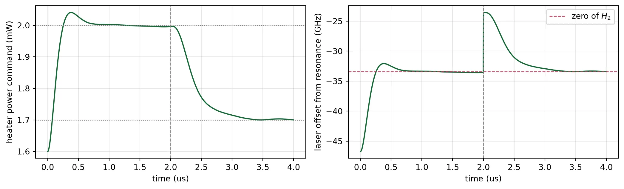
)

time steps                     39368000
laser offset before the step   -33.54 GHz (zero of H2: -33.43 GHz)
laser offset at the end        -33.36 GHz
heater command change          -0.294 mW (step: +0.300 mW)

The integrator brings the heater from 1.6 mW to the operating point in about 1 us and holds it there. The laser settles 33.5 GHz below the resonance, against 33.4 GHz from the transmission curve; the remaining difference comes from the photodiode noise, which the integrator averages. After the step, the integrator lowers the heater power by the added 0.3 mW, and the ring returns to the same operating point. Times in this simulation are about 16,000 times shorter than on the chip, where the same acquisition takes about 20 ms.

All 24 loops together

Dither frequencies

Each heater is dithered at its own frequency, which its lock-in amplifier must be able to separate from every other signal on the same photodiode.

• Monitor photodiode (transmit bank). It receives the dither frequencies $f_1$ to $f_8$ of the eight modulators and their second harmonics. Each modulator loop measures at $2 f_i$, so no $2 f_i$ may coincide with any other $f_j$ or $2 f_j$. This holds if the highest $f_i$ is less than twice the lowest, because then every second harmonic is above every fundamental.
• Channel photodiodes (receive side). Each receives the two dither frequencies of its own filter, $f_A$ and $f_B$, and also the dither of the modulator that produced the channel, which travels with the light. Every channel has its own photodiode, so all eight filters can use the same $f_A$ and $f_B$, chosen away from the modulator frequencies.
• All dither frequencies are below the heater’s 18 kHz corner frequency, so that they reach the rings.

The cell below chooses the frequencies and finds the smallest separation between a measured frequency and any other signal on the same photodiode.

# Dither frequency of each modulator heater (Hz)
mod_tones = np.linspace(3.0e3, 5.5e3, n_channels)

# Dither frequencies of a filter's two heaters (Hz)
filter_tones = np.array([1.2e3, 1.9e3])
lockin_bw = 20.0  # Bandwidth of each lock-in output (Hz)

# Monitor photodiode: modulator frequencies and second harmonics, measured at 2 f_i
monitor = np.concatenate([mod_tones, 2 * mod_tones])
gap_monitor = min(
    np.min(np.abs(np.delete(monitor, n_channels + i) - 2 * f))
    for i, f in enumerate(mod_tones)
)

# Channel photodiode: filter frequencies, their products, and the modulator frequency
fa, fb = filter_tones
gap_channel = np.inf
for f_mod in mod_tones:
    # List the signals on a channel photodiode, for each modulator frequency in turn
    present = np.array([2 * fa, 2 * fb, fa + fb, fb - fa, f_mod, 2 * f_mod])
    for f_read, other in ((fa, fb), (fb, fa)):
        gap_channel = min(
            gap_channel, np.min(np.abs(np.append(present, other) - f_read))
        )

# Calculate how much the highest dither frequency is reduced by the heater response
loss_db = 10 * np.log10(1 + (mod_tones.max() / f_thermal) ** 2)

print(
    f"modulator dithers        {mod_tones.min()*1e-3:.1f} to "
    f"{mod_tones.max()*1e-3:.1f} kHz"
)
print(f"filter dithers           {fa*1e-3:.1f} and {fb*1e-3:.1f} kHz, on every channel")
print(
    f"smallest separation      {gap_monitor:.0f} Hz on the monitor photodiode, "
    f"{gap_channel:.0f} Hz on a channel photodiode"
)
print(f"lock-in bandwidth        {lockin_bw:.0f} Hz")
print(f"highest dither reduced   {loss_db:.2f} dB by the heater response")

modulator dithers        3.0 to 5.5 kHz
filter dithers           1.2 and 1.9 kHz, on every channel
smallest separation      500 Hz on the monitor photodiode, 500 Hz on a channel photodiode
lock-in bandwidth        20 Hz
highest dither reduced   0.37 dB by the heater response

The smallest separation is 500 Hz on both photodiodes, 25 times the 20 Hz bandwidth of the lock-in output, and the highest dither frequency is reduced by 0.4 dB on its way through the heater.

Simulating the loops

Each loop is an integrator: at every time step $\Delta t$ it changes its heater power by $\Delta P = -k \, e \, \Delta t$, where $e$ is the loop’s error signal and $k$ its gain. The loops run at 20 Hz, about 600 times slower than the heater responds, and the lock-in output is an average over many dither periods. The simulation therefore takes the error signals computed above as functions of each ring’s resonance position, instead of simulating the dither waveform itself. It contains:

• modulator error signals: $H_2$ with data, from the previous section;
• filter error signals: the gradient of $\bar{P}$, from the map above;
• thermal coupling: a matrix of the temperature rise of each ring per milliwatt of each heater. It contains the self-heating of each heater, the coupling of $6 \times 10^{-5}$ between rings 150 um apart from the thermal page, and the fraction shared between the two racetracks of a filter, measured above;
• integrator gains chosen so that every loop has a bandwidth of 20 Hz.

The simulation starts from the open-loop calibration: each ring receives a random fabrication offset drawn from the measured spread, and the heater powers are set so that every ring is on its target. A heater can only heat, so it compensates a warmer package by reducing its power. The laser frequency is therefore chosen so that the heater with the lowest power still has enough power to compensate the largest temperature rise studied on this page, 8 K. The shared heating inside each filter is included in this choice.

The package temperature then rises by 4 K in 2 s, once with the loops open and once with them closed.

n_heaters = 3 * n_channels  # One heater per modulator, two per filter
is_mod = np.arange(n_heaters) < n_channels  # Which heaters belong to modulators

# Filter racetrack temperature rise per heater power, measured above (K/mW)
k_filter = rise_a / (p_probe * 1e3)
ghz_per_mw_filter = k_filter * ghz_per_k_strip  # Filter racetrack tuning (GHz/mW)

# Build the thermal matrix: coupling at 150 um, then each heater's own rise
z_th = np.full((n_heaters, n_heaters), coupling * k_per_mw)
np.fill_diagonal(z_th, np.where(is_mod, k_per_mw, k_filter))

# Add the heat shared between the two racetracks of each filter
for i in range(n_channels):
    ha, hb = n_channels + 2 * i, n_channels + 2 * i + 1
    z_th[ha, hb] = z_th[hb, ha] = intra * k_filter

# Give each heater its ring's tuning, rib for modulators and strip for filters (GHz/K)
ghz_per_k = np.where(is_mod, ghz_per_k_rib, ghz_per_k_strip)

# Tabulate the modulator error signal: H2 of the data-averaged transmission
x_table = np.arange(-200.0, 100.0, 0.25)
h_table = np.array([harmonics(t_data, xl, dither * np.sin(phase)) for xl in x_table])
err_raw = h_table[:, 1]

# Keep H2 / H1 as well, limited as a real divider output would be
err_ratio = np.clip(h_table[:, 1] / h_table[:, 0], -1.0, 1.0)

# Interpolate the filter gradient over both racetrack offsets, zero outside the map
filter_grad = [
    RegularGridInterpolator((grid, grid), g, bounds_error=False, fill_value=0.0)
    for g in (grad_a, grad_b)
]

f_loop = 20.0  # Bandwidth of every loop (Hz)
dt_loop = 1e-3  # Loop update interval (s)

# Set the modulator gain from the slope of its error signal at the zero
slope_mod = np.interp(null_data + 0.5, x_table, err_raw) - np.interp(
    null_data - 0.5, x_table, err_raw
)
k_mod = 2 * np.pi * f_loop / (ghz_per_mw_rib * slope_mod)

# Set the gain for H2 / H1 in the same way
slope_ratio = np.interp(null_data + 0.5, x_table, err_ratio) - np.interp(
    null_data - 0.5, x_table, err_ratio
)
k_mod_ratio = 2 * np.pi * f_loop / (ghz_per_mw_rib * slope_ratio)

# Set the filter gain from the second derivative of the mean power at the centre
curv = (surface[mid + 1, mid] - 2 * surface[mid, mid] + surface[mid - 1, mid]) / (
    grid[1] - grid[0]
) ** 2
k_fil = 2 * np.pi * f_loop / (abs(curv) * ghz_per_mw_filter**2)

headroom_k = 8.0  # Largest package warming the loops must compensate (K)

# Draw a fabrication offset for every ring
rng = np.random.default_rng(seed=3)
spread_draw = rng.normal(0, sigma_ring, n_heaters)

# Find the heater powers the offsets alone need, and what a common 1 GHz shift adds
p_spread = np.linalg.solve(z_th, spread_draw / ghz_per_k)
p_pull = np.linalg.solve(z_th, np.ones(n_heaters) / ghz_per_k)

# Find the power each heater must give back if the package warms by the full headroom
reserve = headroom_k * np.linalg.solve(z_th, np.ones(n_heaters))

# Choose the laser position so the heater with the least power still holds that reserve
pull = np.max((reserve - p_spread) / p_pull)

# Resonance of each ring above its target before trimming (GHz)
cold = pull + spread_draw

# Open-loop calibration that puts every ring on its target (mW)
p_cal = p_spread + pull * p_pull

def run_loops(ambient, duration, closed=True, ratio=False):
    """Step all 24 loops in time and return each ring's offset from its target (GHz).

    ambient is a function of time giving the package temperature change (K).
    """
    p = p_cal.copy()  # Start every heater at its calibrated power (mW)
    history = []  # Ring offsets at every step

    # Step through time at the loop update interval
    for t in np.arange(0.0, duration, dt_loop):
        # Find each ring's resonance relative to its target
        offset = cold - ghz_per_k * (z_th @ p + ambient(t))
        history.append(offset.copy())

        # Keep the heater powers fixed when the loops are open
        if not closed:
            continue

        # Read the modulators: laser offset is the target zero minus the ring's offset
        e_mod = np.interp(
            null_data - offset[is_mod], x_table, err_ratio if ratio else err_raw
        )

        # Read the two lock-in outputs of every filter at its racetracks' offsets
        pairs = offset[~is_mod].reshape(-1, 2)
        e_fil = np.stack([g(pairs) for g in filter_grad], axis=1).reshape(-1)

        # Integrate: the modulators drive H2 to zero, the filters follow the gradient
        k_this = k_mod_ratio if ratio else k_mod
        p[is_mod] -= dt_loop * k_this * e_mod
        p[~is_mod] -= dt_loop * k_fil * ghz_per_mw_filter * e_fil

        # Keep the heater powers physical: a heater cannot cool
        np.clip(p, 0.0, None, out=p)
    return np.array(history), p

ramp_k = 4.0  # Package temperature rise (K)
ramp_s = 2.0  # Duration of the rise (s)

def ramp(t):
    """Package temperature change: a steady rise, then constant."""
    return ramp_k * min(t / ramp_s, 1.0)

# Run the temperature rise once with the loops open and once with them closed
open_hist, _ = run_loops(ramp, 3.0, closed=False)
closed_hist, p_end = run_loops(ramp, 3.0, closed=True)
t_axis = np.arange(len(closed_hist)) * dt_loop  # Time axis (s)

fig, ax = plt.subplots(1, 2, figsize=(11, 3.6), sharey=True, tight_layout=True)
for a, hist, title in (
    (ax[0], open_hist, "loops open"),
    (ax[1], closed_hist, "loops closed"),
):
    a.plot(t_axis, hist[:, is_mod], color="#1f4e79", lw=0.8)
    a.plot(t_axis, hist[:, ~is_mod], color="#3aa596", lw=0.8)
    a.set(xlabel="time (s)", title=title)
    a.grid(alpha=0.3)
ax[0].set_ylabel("ring offset from target (GHz)")
ax[0].plot([], [], color="#1f4e79", label="modulators")
ax[0].plot([], [], color="#3aa596", label="filter racetracks")
ax[0].legend(fontsize=8)
plt.show()

print(
    f"calibrated heater power   {p_cal[is_mod].mean():.2f} mW average on the modulators, "
    f"{p_cal[~is_mod].mean():.2f} mW on the filter racetracks"
)
print(f"after a {ramp_k:.0f} K rise in {ramp_s:.0f} s:")
print(f"  loops open     largest offset {np.abs(open_hist[-1]).max():6.2f} GHz")
print(
    f"  loops closed   largest offset {np.abs(closed_hist[-1]).max():6.2f} GHz at the end, "
    f"{np.abs(closed_hist).max():.2f} GHz during the rise"
)
print(f"  heater power   {p_cal.sum():.1f} mW before, {p_end.sum():.1f} mW after")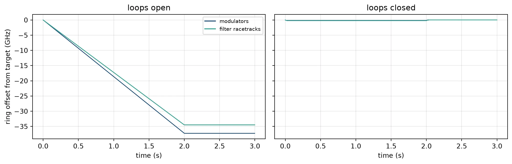

calibrated heater power   5.32 mW average on the modulators, 3.89 mW on the filter racetracks
after a 4 K rise in 2 s:
  loops open     largest offset  37.25 GHz
  loops closed   largest offset   0.00 GHz at the end, 0.25 GHz during the rise
  heater power   104.9 mW before, 85.4 mW after

With the loops open, every ring follows the package temperature and ends 34 to 37 GHz from its target. For the modulators this is most of the distance to the resonance. With the loops closed, every ring stays within 0.25 GHz of its target during the rise and returns to it afterwards. The heaters reduce their total power from 105 mW to 86 mW to compensate the warmer package. The remaining error during the rise is proportional to the rate of the temperature change and inversely proportional to the loop bandwidth.

The reserve for an 8 K rise raises the heater powers: the modulators average 5.4 mW, against 4.2 mW for the open-loop trim on the thermal page, which has no reserve. A design that expects a smaller temperature range can place the laser closer to the resonances and use less power.

The loops do not disturb each other. The coupling between rings 150 um apart is too small to matter. The heat shared between the two racetracks of a filter is handled by its two loops together: each loop measures the slope along its own heater, and that measurement already includes the heat arriving from the other heater.

Recovery from a sudden temperature step

A slow temperature change keeps every ring close to its target. A sudden step, for example when a neighbouring chip is switched on, can move a ring far from its target before the loop reacts. The loop recovers only if the error signal still has the correct sign at that position.

For the modulator, $H_2$ has the correct sign from the operating point up to its next zero, which lies on the other side of the resonance. A ring moved beyond that zero is pulled to the wrong side of the resonance.

Some controllers divide $H_2$ by $H_1$, so that the loop gain does not depend on the optical power. $H_1$ is zero at the transmission minimum, so the ratio changes sign there, and the recovery range then ends at the transmission minimum. The cell below applies temperature steps of increasing size to the locked chip and records whether every modulator returns to its target, for both error signals.

# Find where H1 changes sign above the operating point: the transmission minimum
h1_side = h_table[:, 0][x_table > null_data]
x_side = x_table[x_table > null_data]
x_pole = x_side[np.flatnonzero(np.diff(np.sign(h1_side)))[0]]

# Find the next zero of H2 beyond the transmission minimum
x_far = null(t_data, dither * np.sin(phase), lo=x_pole + 0.5, hi=90.0)

print(f"{'step K':>7s} {'shift GHz':>10s} {'H2 / H1':>9s} {'H2':>9s}")

# Apply each step size with both modulator error signals
for step_k in (2.0, 3.0, 4.0, 5.0, 6.0, 8.0):
    row = []
    for use_ratio in (True, False):
        # Apply the step at time zero and let the loops settle
        hist, _ = run_loops(lambda t: step_k, 1.5, ratio=use_ratio)

        # Count the lock as held if every modulator returns within 2 GHz of its target
        worst = np.abs(hist[-1][is_mod]).max()
        row.append("held" if worst < 2.0 else "lost")
    print(f"{step_k:7.1f} {-step_k*ghz_per_k_rib:10.1f} {row[0]:>9s} {row[1]:>9s}")

print()
print(
    f"transmission minimum  {x_pole - null_data:5.1f} GHz above the operating point, "
    f"{(x_pole - null_data)/ghz_per_k_rib:.1f} K"
)
print(
    f"next zero of H2       {x_far - null_data:5.1f} GHz above the operating point, "
    f"{(x_far - null_data)/ghz_per_k_rib:.1f} K"
)

 step K  shift GHz   H2 / H1        H2
    2.0      -18.6      held      held
    3.0      -27.9      held      held
    4.0      -37.2      lost      held
    5.0      -46.6      lost      held
    6.0      -55.9      lost      held
    8.0      -74.5      lost      lost

transmission minimum   34.1 GHz above the operating point, 3.7 K
next zero of H2        68.5 GHz above the operating point, 7.4 K

With $H_2$ the loops recover from steps up to 6 K and fail at 8 K, as expected from the next zero of $H_2$, 7.4 K above the operating point. With $H_2 / H_1$ they fail from 4 K on, because the transmission minimum is only 3.7 K away. The loops on this page therefore use $H_2$ without dividing by $H_1$. Their gain then changes with the received optical power, but a change of a few decibels only changes the loop bandwidth by the same factor, which the integrator tolerates.

Eye diagrams with the loops open and closed

The cell below transmits 100 Gb/s data through one channel, consisting of a modulator, a drop filter and a photodiode. It uses the same bit pattern, edge rate and eye quality measure, the Q factor, as Link Simulation. The heater settings enter the models as ring temperatures. Three cases are compared:

• Locked: both rings at their operating points. With the loops closed the rings stay there when the package temperature changes, within the recovery range above.
• Package 2 K warmer, loops open: the heaters keep their powers.
• Package 4 K warmer, loops open: the same, for the 4 K rise simulated above.

ui = int(round(1 / bit_rate / dt))  # Samples per bit, at the time step set above

n_pattern = 31  # Bits in one period of the drive pattern
n_reps = 3  # Periods per run
n_steps = n_reps * n_pattern * ui  # Total time steps per run
rise_steps = max(1, int(round(0.3 * ui)))  # Rise and fall time, in steps

def prbs5(shift=0):
    """Generate the 31 bit maximal sequence of x^5 + x^3 + 1, rotated by shift."""
    reg, out = 0x1F, []
    for _ in range(n_pattern):
        bit = ((reg >> 4) ^ (reg >> 2)) & 1
        reg = ((reg << 1) | bit) & 0x1F
        out.append(bit)
    return np.roll(np.array(out), shift)

def nrz(bits):
    """Convert a bit sequence to a drive waveform with finite edges."""
    # Hold each bit for one symbol period, then smooth the steps into ramps
    level = np.repeat(np.tile(bits, n_reps), ui).astype(float)
    return np.convolve(level, np.ones(rise_steps) / rise_steps, mode="same") * v_drive

def eye_fold(v):
    """Fold a trace into overlapping two-bit segments for an eye diagram."""
    # Slide the window one bit at a time, so every transition lands mid trace
    n = len(v) // ui - 1
    return np.stack([v[k * ui : (k + 2) * ui] for k in range(n)])

def eye_q(v, bits, max_lag=24, instant=False):
    """Measure eye quality: level separation over level spread."""
    # Cut the trace into symbol periods, and line up the bits that were sent
    keep = len(v) // ui
    blocks = v[: keep * ui].reshape(-1, ui)
    sent_all = np.tile(bits, n_reps)[-keep:]

    # Search the sampling instant and the whole-bit delay together
    best, best_k = 0.0, 0
    for lag in range(max_lag):
        sent = np.roll(sent_all, lag)
        hi, lo = blocks[sent == 1], blocks[sent == 0]
        if len(hi) < 2 or len(lo) < 2:
            continue
        q = np.abs(hi.mean(axis=0) - lo.mean(axis=0)) / (
            hi.std(axis=0) + lo.std(axis=0) + 1e-18
        )
        k = int(np.argmax(q))
        if q[k] > best:
            best, best_k = float(q[k]), k
    return (best, best_k) if instant else best

# Warm both rings by the average trim, and put the laser at the locked offset
warm = mean_mw * k_per_mw
f_laser = f0 + (null_data - ghz_per_k_rib * warm) * 1e9

# Warm the filter until its passband is centred on that laser line
warm_filter = (f0 - f_laser) * 1e-9 / ghz_per_k_strip

# Generate the bit pattern and the drive waveform
bits = prbs5()
drive = nrz(bits)

def drive_channel(t_mod, t_fil):
    """Send data through modulator, filter and photodiode; return the detected trace."""
    # Build the two rings at the given temperatures
    mod = microring_modulator(**{**mrm.parametric_kwargs, "temperature": t_mod})
    fil = two_ring_filter(**{**second_order.parametric_kwargs, "temperature": t_fil})

    # Pass the laser through the modulator, with the drive on its electrical port
    ts = mod.setup_time_stepper(time_step=dt, carrier_frequency=f_laser)
    laser = np.full(n_steps, np.sqrt(p_line), dtype=complex)  # Laser at constant power
    out = ts.step(
        inputs=pf.TimeSeries({"P0@0": laser, "E0@0": drive / sq}, dt),
        show_progress=False,
    )

    # Pass the modulated light through the filter, to its drop port
    ts = fil.setup_time_stepper(time_step=dt, carrier_frequency=f_laser)
    out = ts.step(inputs=pf.TimeSeries({"in@0": out["P1@0"]}, dt), show_progress=False)

    # Detect the dropped light, and discard the first period while the resonators fill
    ts = pd.setup_time_stepper(time_step=dt, carrier_frequency=f_laser)
    out = ts.step(
        inputs=pf.TimeSeries({"P0@0": out["drop@0"]}, dt), show_progress=False
    )
    return (np.real(out["E0@0"]) * sq)[n_pattern * ui :]

# Set the ring temperatures: locked, then the package warmer with the heaters unchanged
cases = {
    "locked": (t_ref + warm, t_ref + warm_filter),
    "+2 K, loops open": (t_ref + warm + 2.0, t_ref + warm_filter + 2.0),
    "+4 K, loops open": (t_ref + warm + 4.0, t_ref + warm_filter + 4.0),
}

t_eye = (np.arange(2 * ui) - ui) * dt * 1e12  # Time axis of the eye (ps)
fig, ax = plt.subplots(1, 3, figsize=(13, 3.6), sharey=True, tight_layout=True)
for a, (label, temps) in zip(ax, cases.items()):
    # Send the data through the channel, then fold the trace at the best sampling time
    trace = drive_channel(*temps)
    q, k = eye_q(trace, bits, instant=True)
    a.plot(
        t_eye, eye_fold(np.roll(trace, -k)).T * 1e3, color="#1f4e79", alpha=0.25, lw=0.7
    )
    a.set_title(f"{label}\nQ = {q:.2f}", fontsize=9)
    a.set_xlabel("time (ps)")
    a.grid(alpha=0.3)
ax[0].set_ylabel("detected (mV)")
plt.show()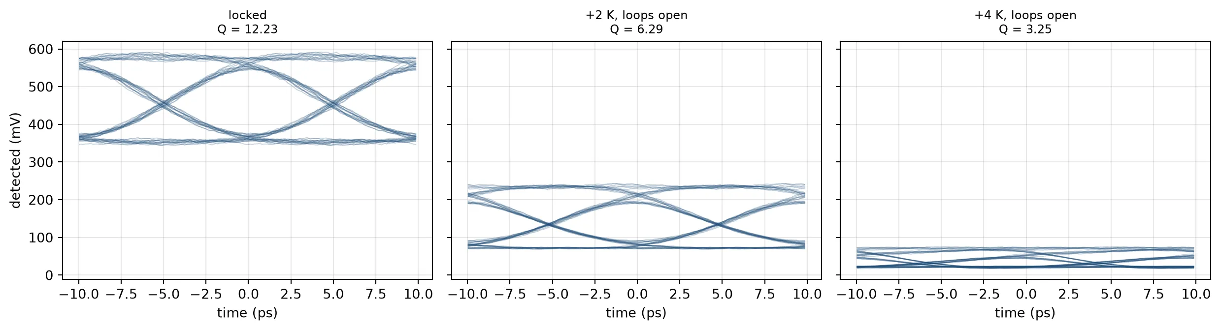

In the locked case the eye is open. With the package 2 K warmer and the loops open, the modulator is closer to its resonance and the filter passband is off the carrier: the detected signal drops to less than half, and the Q factor is halved. At 4 K the eye is nearly closed. With the loops closed, the channel keeps the first eye during the 4 K rise simulated above.

Summary

	drop filter	ring modulator
target	passband centred on the carrier	inflection point of the data-averaged transmission
photodiode	the channel’s own photodiode	one monitor photodiode for eight modulators
heaters	two, one per racetrack	one
error signal	first harmonic of each heater’s dither	second harmonic of the heater’s dither
why it works	with 100 Gb/s data the passband centre is a maximum	its zero does not depend on the optical power
dither applied to	heater power	heater power

Three results apply to other ring circuits as well:

• The error signal depends on what the photodiode averages. For a flat passband, a CW probe and 100 Gb/s data give opposite signs of the second derivative at the passband centre.
• An error signal that is zero at the target needs no reference value. This is what allows one photodiode to serve eight modulators, regardless of the light level on it.
• A heater is a square-law actuator. A dither applied to its voltage creates a second harmonic of its own, so the dither is applied to the heater power.