LiDAR Beam Steering and Thermal Budget

Download notebook (.zip)

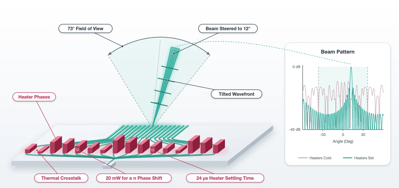
The chip layout page left a phased array in which every cell carries a model, and the antenna page saved the radiation pattern of each antenna. This notebook puts the two together and answers five questions: where the beam points, how wide it is, how far it can be steered before a grating lobe takes over, what the heaters have to do to point it, and what that costs in milliwatts and in microseconds.

The chain runs in four steps.

• The feed network is asked for the amplitude and phase it delivers to each of the 32 antennas, as drawn, with every heater cold. That is a circuit S matrix of the drawn cell.
• An FDTD run of eight antennas side by side, against one of a single antenna in the same domain, measures what the neighbours do to the spectrum of the light an antenna radiates.
• Those 32 complex amplitudes multiply the element pattern into the beam the array forms, and the heater phases that point it anywhere in the field of view follow by construction.
• Heat solves of the phase shifter give the power a radian costs, how much of it leaks to the neighbouring channels, and how long the heater takes to settle, which is the steering rate.

The page closes with the power budget, a fabrication sensitivity table, and a file of heater settings against beam angle and wavelength for the ranging page.

Lidar_Chip.qmd

# The feed cell, the chip, the antenna numbers and the technology come from
from runpy import run_path

# Lidar_Chip.qmd defines what this notebook builds on. Its shared cells are
# generated into the module below; see docs/scripts/generate_notebook_modules.py.
globals().update(
    {k: v for k, v in run_path("misc/lidar_chip.py").items() if not k.startswith("_")}
)

from tidy3d import web

# Open the layout viewer for the sub-array built below
viewer = LiveViewer()

# The antennas' spectrum and cuts, saved by Lidar_Antenna.qmd
far = np.load("misc/element_far_field.npz")
# radiated power against (kx/k0, ky/k0) at 1550 nm, 500 nm antenna alone
spectrum_alone = far["spectrum"]
# lateral angle in air on the cut through the peak (deg)
theta_lateral = far["theta_lateral"]
# element pattern of the 500 nm antenna alone
element_alone = far["lateral"] / far["lateral"].max()
# longitudinal emission angle at each wavelength (deg)
peak_angle = far["peak_angle"]

# Antenna positions across the array, from the array cell
y_ant = np.array([antenna_array.ports[f"A{k}"].center[1] for k in range(n_ch)])

# Lateral angle grid of the far field (deg)
theta = np.linspace(-90, 90, 3601)

LiveViewer started at http://127.0.0.1:36231. Call its 'stop()' method to free the port.

The feed as built

The circuit model of the feed cell composes 31 splitters, 63 S bends, 32 phase shifters and 32 fan-in bends into one S matrix from the input to the 32 antenna ports. Each entry is the amplitude and phase one channel delivers, with the heaters cold. The amplitudes should be equal, since the tree is balanced. The phases are not: the layout page recorded that the fan-in makes the outer channels up to 132 um longer, and that length appears here as phase, hundreds of turns of it, of which only the fraction of a turn is visible. The phase the recorded paths predict from the strip index is drawn for comparison, and what is left after it is removed is printed.

# S matrix of the feed, from its input to the 32 antenna ports, across the tuning range
s_feed = feed.s_matrix(freqs, model_kwargs={"inputs": ["IN"]}, show_progress=False)

# Complex amplitude at each antenna and each wavelength, indexed (wavelength, channel)
a_built = np.array(
    [[s_feed[("IN@0", f"A{k}@0")][i] for k in range(n_ch)] for i in range(len(freqs))]
)

# Power reaching the antennas together, and its spread across channels, at the design wavelength
power = np.abs(a_built[i0]) ** 2
print(
    f"power delivered to the 32 antennas: {10 * np.log10(power.sum()):.2f} dB of the input, "
    f"channel spread {10 * np.log10(power.max() / power.min()):.2f} dB"
)

# Phase as built, wrapped to one turn, and the phase the recorded paths predict, referred to
# the centre channel. A phase is only known modulo a turn, so both are shown wrapped.
centre_phase = a_built[i0, n_ch // 2] / abs(a_built[i0, n_ch // 2])
phase_built = np.angle(a_built[i0])
phase_path = np.angle(
    np.exp(2j * np.pi * n_eff_strip * (path - path[n_ch // 2]) / lda0) * centre_phase
)

# What is left once the path phase is removed: the splitters and bends, identical for every channel
residual = np.angle(
    a_built[i0]
    * np.exp(-2j * np.pi * n_eff_strip * (path - path[n_ch // 2]) / lda0)
    / centre_phase
)
print(
    f"phase left after removing the recorded paths: {np.degrees(np.abs(residual).max()):.1f} deg at most"
)

fig, ax = plt.subplots(1, 2, figsize=(11, 4))
ax[0].plot(range(n_ch), 10 * np.log10(power), "o")
ax[0].set_xlabel("channel")
ax[0].set_ylabel("power at the antenna (dB)")
ax[0].set_title("amplitude as built")
ax[1].plot(range(n_ch), phase_built, "o", label="feed S matrix")
ax[1].plot(range(n_ch), phase_path, "x", label="from the recorded paths")
ax[1].set_xlabel("channel")
ax[1].set_ylabel("phase, wrapped (rad)")
ax[1].set_title("phase as built at 1550 nm")
ax[1].legend()
plt.tight_layout()
plt.show()

power delivered to the 32 antennas: -0.66 dB of the input, channel spread 0.03 dB
phase left after removing the recorded paths: 0.0 deg at most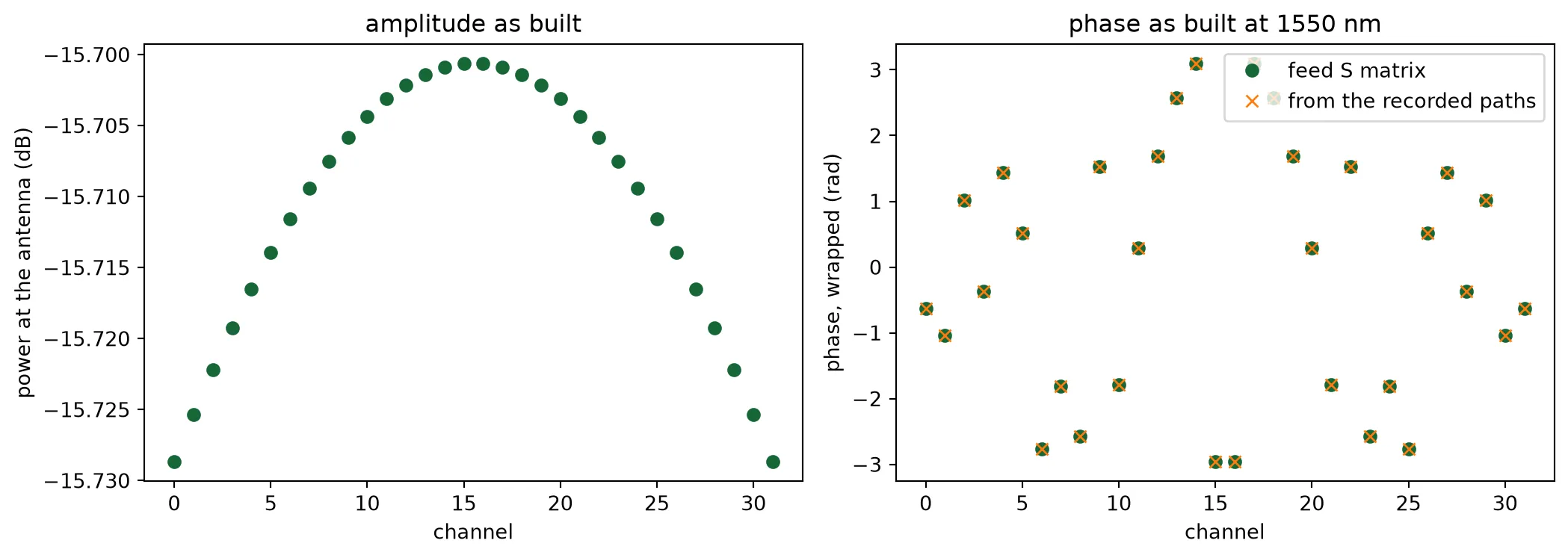

The antenna in the array

The antenna page measured each antenna alone and inside a row of three with the widths alternating. The array has thirty-two, so the check here is a row of eight at the array pitch, widths alternating, with the fifth antenna fed, in the same window and on the same mesh as the antenna page’s runs. The transmission into the other seven antennas’ outputs is the crosstalk, and the spectrum of the fed antenna inside the row is laid over the spectrum of the same antenna alone and inside the row of three, in the three views the antenna page introduced. If seven neighbours do what two did, the two embedded patterns of the antenna page stand for the whole array.

n_sub = 8  # Antennas in the test array
fed = n_sub // 2  # The one that is driven: a 500 nm antenna, on an even position

# Eight sections at the array pitch, widths alternating as in the array, in the antenna page's window
widths = list(antenna_design)
sub = antenna_row(
    [antenna_design[widths[k % 2]]["cell"] for k in range(n_sub)], "sub_array"
)
print(
    f"sub-array {sub.size()[0]:.0f} x {sub.size()[1]:.1f} um, {len(sub.ports)} ports, "
    f"in the same {2 * half_width:.0f} um window as the antenna page's runs"
)
viewer(sub)

sub-array 20 x 11.1 um, 16 ports, in the same 20 um window as the antenna page's runs

LayoutSchematic

# Power out of every antenna's far end, relative to the fed one's; the row of eight is the only
# new run, the single antenna and the row of three come from the antenna page's cache
s_sub = sub.s_matrix([f0], model_kwargs={"inputs": [f"IN{fed}"]}, show_progress=False)
through = np.array(
    [abs(s_sub[(f"IN{fed}@0", f"OUT{k}@0")][0]) ** 2 for k in range(n_sub)]
)
back = np.array([abs(s_sub[(f"IN{fed}@0", f"IN{k}@0")][0]) ** 2 for k in range(n_sub)])
s_lone = lone.s_matrix([f0], model_kwargs={"inputs": ["IN0"]}, show_progress=False)
print(
    f"fed antenna transmits {through[fed]:.3f} of its input, against "
    f"{abs(s_lone[('IN0@0', 'OUT0@0')][0]) ** 2:.3f} alone"
)
print("antenna   forward (dB)   backward (dB)")
for k in range(n_sub):
    print(
        f"  {k}  {'fed' if k == fed else '   '}   {10 * np.log10(through[k] / through[fed]):8.1f}      "
        f"{10 * np.log10(max(back[k], 1e-12) / through[fed]):8.1f}"
    )

# Power reaching the air, with and without neighbours
flux = {}
for name, cell, port in (("in the array", sub, f"IN{fed}"), ("alone", lone, "IN0")):
    data = next(
        iter(
            cell.models["FDTD"]
            .batch_data(cell, [f0], inputs=[port], show_progress=False)
            .values()
        )
    )
    flux[name] = float(data["up"].flux.values[0])
print(
    f"radiated into the air: {flux['in the array']:.4f} of the input in the array, {flux['alone']:.4f} alone"
)

# The three views: the 500 nm antenna alone, inside the row of three, and inside the row of eight,
# per unit radiated power and section length as on the antenna page
ux_s, uy_s, power_sub = spectrum(sub, port=f"IN{fed}", frequencies=[f0])
power_sub = power_sub / (
    radiation(sub, f"IN{fed}", f"OUT{fed}")["radiated"] * sub.properties["l_grating"]
)
_, _, power_lone = spectrum(lone, port="IN0", frequencies=[f0])
power_lone = power_lone / (
    radiation(lone, "IN0", "OUT0")["radiated"] * lone.properties["l_grating"]
)
plot_spectrum(
    {
        "alone": (ux_s, uy_s, power_lone[:, :, 0]),
        "between two neighbours": (ux_s, uy_s, embedded["500 nm between 450 nm"][2]),
        "between seven neighbours": (ux_s, uy_s, power_sub[:, :, 0]),
    },
    "the 500 nm antenna alone, in a row of three and in a row of eight, 1550 nm",
)

# Element patterns through the peak, and how far the neighbours move it
_, _, theta_lone, lateral_lone = cuts(ux_s, uy_s, power_lone, i_lda=0)
_, _, theta_sub, lateral_sub = cuts(ux_s, uy_s, power_sub, i_lda=0)
theta_three, lateral_three, _ = embedded["500 nm between 450 nm"]
scale = lateral_lone.max()
print("lateral angle   alone   row of three   row of eight")
for t in (0, 10, 20, 30, 40):
    print(
        f"   {t:3d} deg     {np.interp(t, theta_lone, lateral_lone) / scale:5.2f}      "
        f"{np.interp(t, theta_three, lateral_three) / scale:5.2f}          {np.interp(t, theta_sub, lateral_sub) / scale:5.2f}"
    )

fed antenna transmits 0.966 of its input, against 0.967 alone
antenna   forward (dB)   backward (dB)
  0           -55.7         -88.5
  1           -55.7         -89.5
  2           -56.0         -82.1
  3           -54.0        -102.5
  4  fed        0.0         -35.4
  5           -53.7        -104.5
  6           -54.3         -81.9
  7           -57.0         -91.5
radiated into the air: 0.0178 of the input in the array, 0.0161 alone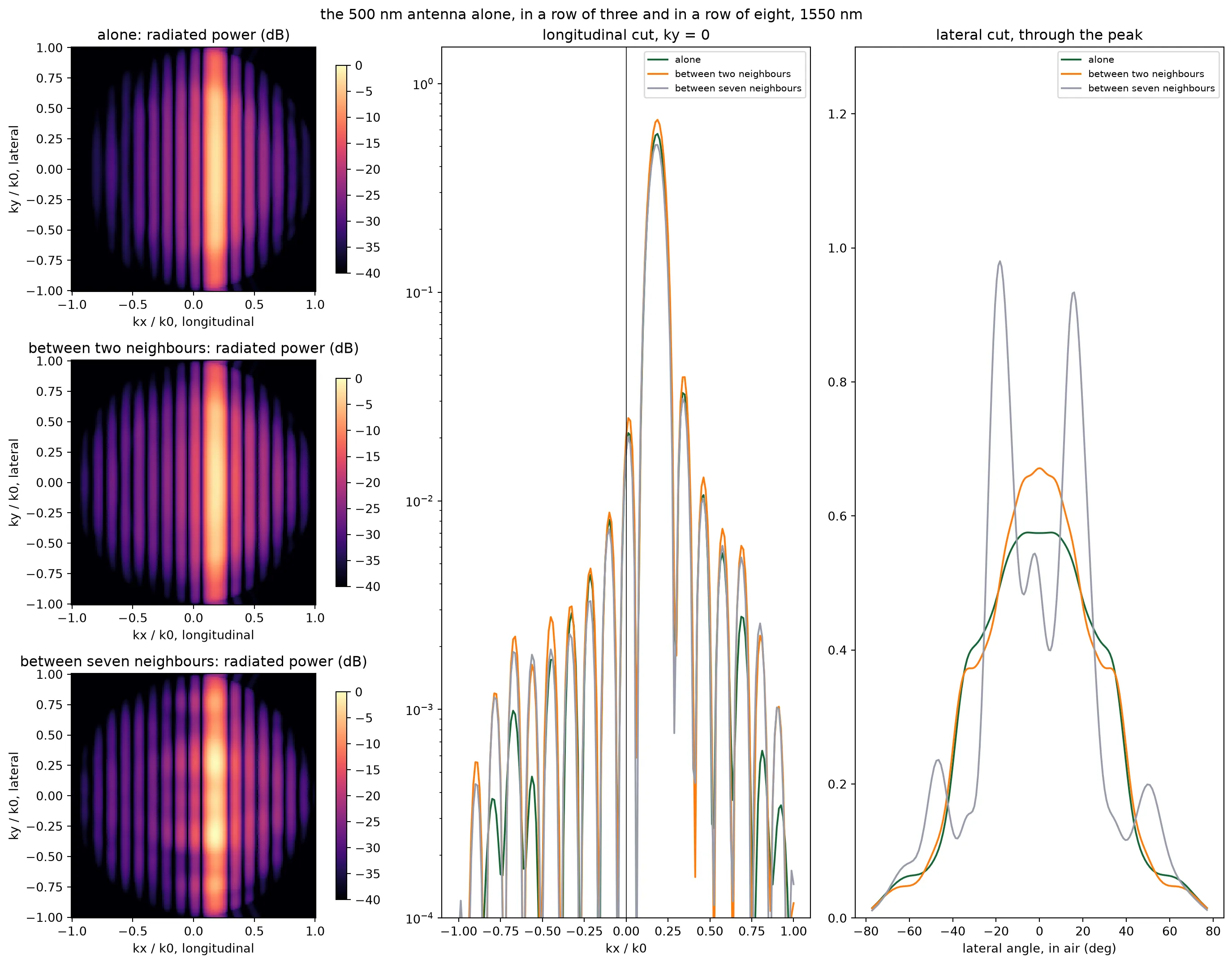

lateral angle   alone   row of three   row of eight
     0 deg      1.00       1.17           0.88
    10 deg      0.98       1.09           1.06
    20 deg      0.82       0.81           1.31
    30 deg      0.71       0.65           0.33
    40 deg      0.40       0.44           0.20

The crosstalk is small: after 30 um the nearest neighbour carries about 50 dB less than the fed antenna, and the fed antenna transmits what it transmits alone. This is the detuning of the alternating widths. The longitudinal spectrum is unchanged too: the stripe sits at the same $k_x$ with the same width and the same sidelobes, because the grating sets $k_x$ and the neighbours do not enter. What the neighbours change is the lateral cut. Strips 0.8 um away catch part of the light that leaves the antenna sideways and send some of it back upward. This puts about ten percent more power into the air and reshapes the pattern: two neighbours raise it by a fifth at normal; seven neighbours lift it by a third at 20 degrees and pull it down to half by 30. The re-radiation of the neighbours is coherent with the antenna’s own, so more neighbours make sharper fringes, and the pattern of the fed antenna changes by up to half the peak between the rows of three and eight. The three views separate the two effects. The grating focuses the light along $k_x$ and the neighbours leave that axis alone. Laterally, in $k_y$, a single antenna focuses nothing; the array factor of thirty-two antennas does.

Every interior antenna sees the same neighbours, so an embedded pattern stands for all of them; only the outermost few see fewer neighbours on one side. The beam below uses the antenna page’s two patterns from the rows of three, one for each width, since those exist for both antennas; the row of eight says how far a full array moves them, and the field-of-view margins below are read with that spread in mind.

# Element pattern of each channel, from the antenna page's rows of three: 500 nm on even channels,
# 450 nm on odd ones, on one scale so an unequal pair would show up as a lobe at lambda / 2d
theta_500, lateral_500, _ = embedded["500 nm between 450 nm"]
theta_450, lateral_450, _ = embedded["450 nm between 500 nm"]
scale = max(lateral_500.max(), lateral_450.max())
element_by_width = np.array(
    [
        np.interp(theta, theta_500, lateral_500 / scale, left=0.0, right=0.0),
        np.interp(theta, theta_450, lateral_450 / scale, left=0.0, right=0.0),
    ]
)
element_by_channel = element_by_width[np.arange(n_ch) % 2]  # (channel, angle)

The beam

An array of $N$ antennas at positions $y_k$, each fed with a complex amplitude $a_k$, radiates against the lateral angle $\psi$ a field proportional to

$$E(\psi) = \sqrt{E_1(\psi)}\, \sum_k a_k\, e^{\,j k_0 y_k \sin\psi},$$

where $E_1$ is the power pattern of one antenna and the sum is the array factor. The beam points where the phases of the terms line up. With the heaters cold they do not: the as-built phase is quadratic across the array, and the beam is smeared. A heater on channel $k$ adds a phase $\varphi_k$, so setting

$$\varphi_k = -\arg a_k - k_0 y_k \sin\psi_0 \pmod{2\pi}$$

cancels the as-built phase and puts a linear ramp in its place, which steers the beam to $\psi_0$. Wrapping to one turn is what keeps every heater within a 2π range.

One convention has to be fixed before any of this is coded: in PhotonForge the phase of a waveguide’s transmission grows with its length, and heating a phase shifter adds to it, so a heater phase $\varphi_k$ multiplies $a_k$ by $e^{j\varphi_k}$ and the setting above carries the signs it does.

k0 = 2 * np.pi / lda0  # Free-space wavenumber at the design wavelength (1/um)

def beam(amps, lda=lda0):
    """Far-field power against the lateral angle for the antenna amplitudes given, normalized to the
    peak an ideal uniform array of the same total power and a unit element pattern would have.
    """
    # Each channel's field: its amplitude, its position phase, and its own element pattern
    phase = np.exp(1j * (2 * np.pi / lda) * np.outer(np.sin(np.radians(theta)), y_ant))
    field = (phase * np.sqrt(element_by_channel).T) @ amps

    # Ideal peak: same total power, equal amplitudes, perfect phase, unit element pattern
    ideal = (np.sqrt(np.sum(np.abs(amps) ** 2) / n_ch) * n_ch) ** 2
    return np.abs(field) ** 2 / ideal

def heater_phases(theta_deg, i_lda=i0):
    """Heater phase per channel that steers the as-built array to theta_deg, wrapped to one turn."""
    phi = -np.angle(a_built[i_lda]) - k0 * y_ant * np.sin(np.radians(theta_deg))
    return np.mod(phi, 2 * np.pi)

def steered(theta_deg, i_lda=i0, phi=None):
    """Antenna amplitudes with the heaters set for theta_deg; heating adds phase in the model."""
    if phi is None:
        phi = heater_phases(theta_deg, i_lda)
    return a_built[i_lda] * np.exp(1j * phi)

def lobes(pattern):
    """Peak angle, full width at half maximum, and the strongest lobe outside the main one, in dB."""
    i_peak = np.argmax(pattern)
    above = pattern > pattern[i_peak] / 2
    # Main-lobe extent: the contiguous run of half-power points around the peak
    lo = i_peak
    while lo > 0 and above[lo - 1]:
        lo -= 1
    hi = i_peak
    while hi < len(theta) - 1 and above[hi + 1]:
        hi += 1
    outside = pattern.copy()
    # Blank the main lobe out to its first nulls before looking for the next lobe
    null_lo = lo - np.argmax(np.diff(pattern[: lo + 1][::-1]) > 0) if lo > 0 else 0
    null_hi = (
        hi + np.argmax(np.diff(pattern[hi:]) > 0)
        if hi < len(theta) - 1
        else len(theta) - 1
    )
    outside[null_lo : null_hi + 1] = 0
    return (
        theta[i_peak],
        theta[hi] - theta[lo],
        10 * np.log10(outside.max() / pattern[i_peak]),
    )

# Three beams: heaters cold, heaters set for broadside, heaters set for 15 degrees
cases = {
    "heaters cold": a_built[i0],
    "set for 0 deg": steered(0.0),
    "set for 15 deg": steered(15.0),
}

fig, ax = plt.subplots(1, 1, figsize=(9, 4.2))
for name, amps in cases.items():
    p = beam(amps)
    peak, fwhm, side = lobes(p)
    print(
        f"{name:14s}: peak at {peak:6.2f} deg, {fwhm:.2f} deg wide, strongest other lobe {side:.1f} dB"
    )
    ax.plot(theta, 10 * np.log10(np.maximum(p, 1e-6)), label=name)
ax.set_xlim(-90, 90)
ax.set_ylim(-40, 2)
ax.set_xlabel("lateral angle (deg)")
ax.set_ylabel("radiated power (dB, ideal peak = 0)")
ax.set_title("lateral beam pattern at 1550 nm")
ax.legend()
plt.show()

heaters cold  : peak at   8.25 deg, 2.55 deg wide, strongest other lobe -0.0 dB
set for 0 deg : peak at   0.00 deg, 1.80 deg wide, strongest other lobe -13.3 dB
set for 15 deg: peak at  15.00 deg, 1.90 deg wide, strongest other lobe -12.0 dB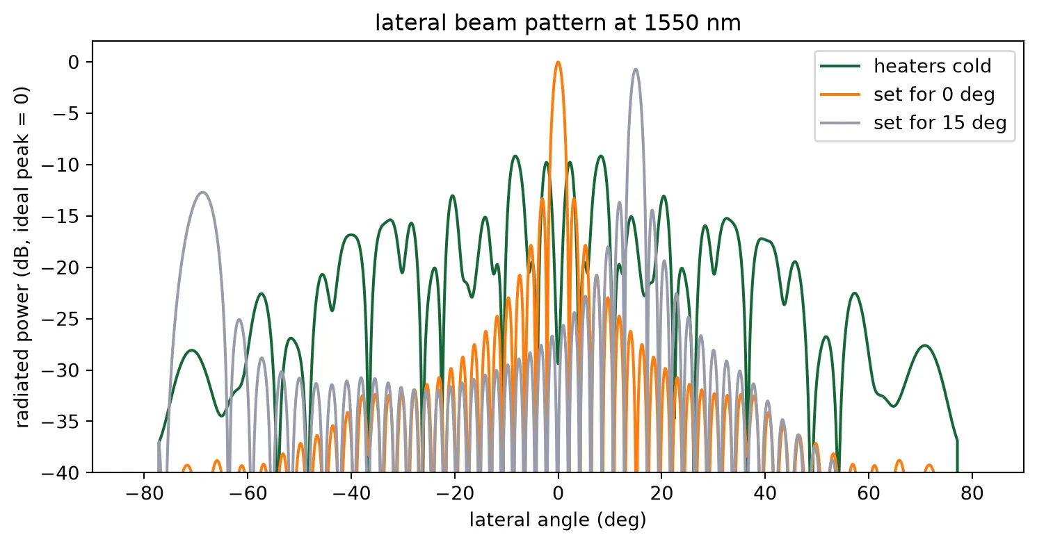

With the heaters cold the array radiates a smear several degrees wide: the quadratic phase of the fan-in acts as a lens with a very short focal length, and the beam never forms. With the heaters set for broadside, the beam is 1.8 degrees wide, close to what a 42 um aperture predicts, with the first sidelobe 13 dB down, which is the value a uniformly fed aperture always gives, and no grating lobe anywhere in the visible half-space: at a 1.3 um pitch the first lobe of a broadside beam would sit beyond the horizon. Set for 15 degrees, the beam is the same shape and the grating lobe has entered at the far edge, where the element pattern leaves it well down. The alternating widths do not show: an unequal pair would radiate a lobe at $\lambda / 2d$, 37 degrees from the beam, and there is none above the sidelobes.

Field of view

Steering the main beam one way moves its grating lobe the other way, and at the edge of the pitch’s unambiguous range, $\pm\arcsin(\lambda / 2d)$, the two swap roles: the lobe that was the grating lobe is now the beam and the scan has, in effect, wrapped around. The field of view is that range, 73 degrees for a 1.3 um pitch. A pitch below the wavelength means that a broadside beam has no grating lobe in the visible half-space at all; the lobe enters at the far edge as the beam steers, and how much weaker it is depends only on the element pattern at the two angles. The sweep below steers across the field of view and records that ratio at every setting.

angles = np.arange(-40.0, 40.1, 1.0)  # Steering angles to sweep (deg)

# For every steering angle: the lobe at the setting, and the strongest lobe anywhere else
sweep = []
for t in angles:
    p = beam(steered(t))
    at_setting = p[np.abs(theta - t) < 1.5].max()
    elsewhere = p[np.abs(theta - t) > 3.0].max()
    sweep.append((theta[np.argmax(p)], 10 * np.log10(elsewhere / at_setting)))
sweep = np.array(sweep)

# Field of view: the pitch's unambiguous range, one beam and one grating lobe inside it
fov_pitch = 2 * np.degrees(np.arcsin(lda0 / (2 * pitch_ant)))
fov = fov_pitch
in_view = np.abs(angles) <= fov / 2
print(f"field of view: 2 asin(lambda / 2d) = {fov:.1f} deg")

# A return through a grating lobe is transmitted and received through it, so it pays the
# one-way ratio twice. Where the ratio is positive the grating lobe is the stronger of the two.
ambiguous = angles[in_view][sweep[in_view, 1] >= 0]
print(
    f"grating lobe against the beam inside the field of view: from {sweep[in_view, 1].min():+.1f} to "
    f"{sweep[in_view, 1].max():+.1f} dB one way, {2 * sweep[in_view, 1].max():+.1f} dB round trip at worst; "
    f"at broadside {sweep[angles == 0, 1][0]:+.1f} dB one way"
)
print(
    f"the grating lobe is the stronger lobe at {len(ambiguous)} of {in_view.sum()} settings"
    + (
        f", from {ambiguous.min():+.0f} to {ambiguous.max():+.0f} deg"
        if len(ambiguous)
        else ""
    )
)

# Eight beams across the field of view, on one axis
fig, ax = plt.subplots(1, 2, figsize=(12, 4.2))
for t in np.arange(-30, 31, 10):
    ax[0].plot(
        theta,
        10 * np.log10(np.maximum(beam(steered(float(t))), 1e-6)),
        label=f"{t:+.0f} deg",
    )
ax[0].set_xlim(-90, 90)
ax[0].set_ylim(-30, 2)
ax[0].set_xlabel("lateral angle (deg)")
ax[0].set_ylabel("radiated power (dB)")
ax[0].set_title("beams across the field of view")
ax[0].legend(fontsize=8, ncol=2)

# The strongest other lobe against steering angle, one way and round trip
ax[1].plot(angles, sweep[:, 1], label="one way")
ax[1].plot(angles, 2 * sweep[:, 1], label="round trip")
for edge in (-fov / 2, fov / 2):
    ax[1].axvline(edge, color="gray", linestyle="--", linewidth=1)
ax[1].axhline(0, color="k", linewidth=0.6)
ax[1].set_xlabel("steering angle (deg)")
ax[1].set_ylabel("strongest other lobe (dB)")
ax[1].set_title("grating lobe against steering")
ax[1].legend()
plt.tight_layout()
plt.show()

field of view: 2 asin(lambda / 2d) = 73.2 deg
grating lobe against the beam inside the field of view: from -13.3 to -0.3 dB one way, -0.5 dB round trip at worst; at broadside -13.3 dB one way
the grating lobe is the stronger lobe at 0 of 73 settings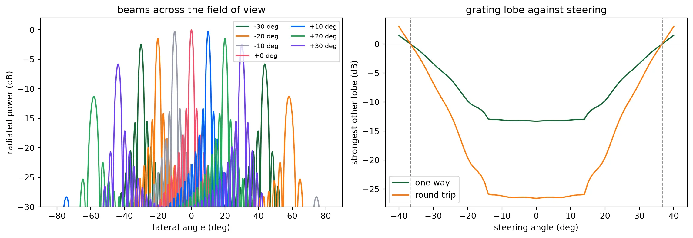

The field of view is the 73 degrees the pitch predicts, and inside it the beam is always the stronger lobe. Near broadside there is no grating lobe at all; as the beam steers out, the lobe enters at the opposite edge where the element pattern is dark, and it approaches the beam only at the very edge of the field of view, where the two are mirror images by symmetry and the ratio must go to zero. Over the central 50 degrees the lobe stays 6 dB or more below the beam one way, and twice that on the round trip, since the receive array has the same pattern and a return through the grating lobe is received through it as well. The sub-wavelength pitch and the partial-etch teeth of the antenna page are what removes the grating lobe. Poulton et al. saw grating lobes with power similar to the main beam on the 2 um pitch chip this design started from, and attributed them to the element factor; the two choices together remove both parts of that problem. The margins here are read from the rows-of-three patterns. The row of eight moves those patterns by up to half the peak between 20 and 30 degrees, so the beam levels there carry an uncertainty of a few decibels, and the edges of the usable range should be read with it.

The second axis is steered by wavelength, and the antenna page measured the emission angle at five wavelengths across the tuning range. The two axes together give the scanned area, drawn below as the grid of beam positions the chip can reach.

# Beam positions: lateral by the heater phases, longitudinal by the wavelength
fig, ax = plt.subplots(1, 1, figsize=(7, 4.5))
for i, lda in enumerate(wavelengths):
    ax.plot(
        angles[in_view],
        np.full(in_view.sum(), peak_angle[i]),
        ".",
        label=f"{lda * 1e3:.0f} nm",
    )
ax.set_xlabel("lateral angle, steered by the heater phases (deg)")
ax.set_ylabel("longitudinal angle, steered by the wavelength (deg)")
ax.set_title(
    f"field of view: {fov:.0f} deg by {peak_angle.max() - peak_angle.min():.0f} deg"
)
ax.legend(fontsize=8)
plt.tight_layout()
plt.show()
print(
    f"scanned field: {fov:.0f} deg lateral, {peak_angle.max() - peak_angle.min():.1f} deg longitudinal, "
    f"about {fov / 1.4:.0f} by {(peak_angle.max() - peak_angle.min()) / np.degrees(lda0 / l_antenna):.0f} beam positions"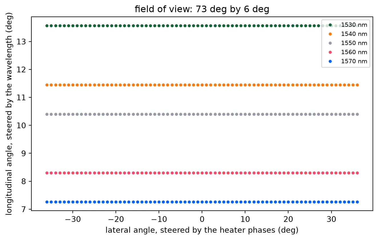
)

scanned field: 73 deg lateral, 6.3 deg longitudinal, about 52 by 75 beam positions

Wavelength and the heater table

The heaters are set from the S matrix at one wavelength. Tune the laser and two things move: the antennas point elsewhere along their length, which is the intended second axis, and the phases across the array change, because the channels differ in length and the light in a longer channel accumulates more phase per nanometre of tuning. The technology page put that at 44 rad for a 100 um mismatch over the tuning range; the fan-in mismatch is 132 um. The heater phase itself also drifts, since a thermo-optic phase is a fixed index change over a fixed length and therefore scales with $1/\lambda$.

Both effects are in the S matrix at each wavelength, so the beam that a fixed heater setting produces at another wavelength follows directly, and so does the setting that wavelength needs.

# Heaters set for broadside at 1550 nm, then held while the laser is tuned
phi_1550 = heater_phases(0.0, i0)
fig, ax = plt.subplots(1, 1, figsize=(9, 4.2))
for i, lda in enumerate(wavelengths):
    # The heater phase is an index change over a length, so it scales with 1/wavelength
    amps = a_built[i] * np.exp(1j * phi_1550 * lda0 / lda)
    p = beam(amps, lda)
    peak, fwhm, side = lobes(p)
    print(
        f"{lda * 1e3:.0f} nm with the 1550 nm setting: peak {10 * np.log10(p.max()):6.1f} dB at {peak:6.2f} deg, "
        f"strongest other lobe {side:.1f} dB"
    )
    ax.plot(theta, 10 * np.log10(np.maximum(p, 1e-6)), label=f"{lda * 1e3:.0f} nm")
ax.set_xlim(-45, 45)
ax.set_ylim(-30, 2)
ax.set_xlabel("lateral angle (deg)")
ax.set_ylabel("radiated power (dB)")
ax.set_title("heaters set at 1550 nm, laser tuned")
ax.legend()
plt.show()

# The table: heater phases for every steering angle at every wavelength
table_angles = np.arange(-30.0, 30.1, 2.0)
phase_table = np.array(
    [[heater_phases(t, i) for t in table_angles] for i in range(len(wavelengths))]
)
print(
    f"\nheater table: {phase_table.shape[0]} wavelengths x {phase_table.shape[1]} angles x {phase_table.shape[2]} channels"
)

1530 nm with the 1550 nm setting: peak  -11.2 dB at -34.45 deg, strongest other lobe -0.1 dB
1540 nm with the 1550 nm setting: peak  -11.5 dB at  12.80 deg, strongest other lobe -0.0 dB
1550 nm with the 1550 nm setting: peak   -0.0 dB at   0.00 deg, strongest other lobe -13.3 dB
1560 nm with the 1550 nm setting: peak  -11.4 dB at -13.00 deg, strongest other lobe -0.0 dB
1570 nm with the 1550 nm setting: peak  -11.7 dB at  35.50 deg, strongest other lobe -0.1 dB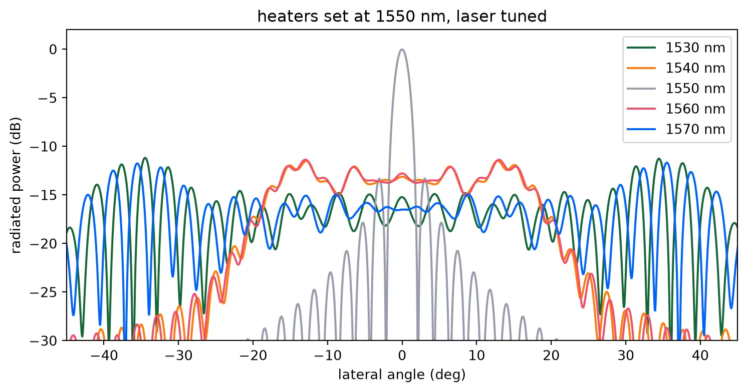

heater table: 5 wavelengths x 31 angles x 32 channels

Ten nanometres of tuning degrades the beam, and twenty destroys it. The layout page showed that the path lengths cannot be matched in this geometry, so the remedy is a table: one set of 32 heater phases per steering angle per wavelength, computed here from the drawn chip rather than measured. Optical phased arrays are calibrated into such a table, and the ranging page drives the chip with it.

Phase errors and calibration

Fabrication puts a random phase on every channel. The strip index moves by about 10⁻³ per nanometre of width, so over the two millimetres from the input to an antenna a one nanometre width error between two channels is several radians. No phased array works uncalibrated, and the table above is really the design part of a calibration that a fabricated chip completes by measurement. What matters for the design is the residual: how well the heaters have to be set, and what the beam loses when they are set imperfectly. The Monte Carlo below adds a random phase of a given standard deviation to every channel and reads the beam.

rng = np.random.default_rng(1)
sigmas = (0.05, 0.15, 0.3, 0.6)  # Residual phase error per channel (rad)
n_trials = 200

ideal = steered(0.0)
# the beam with no error, which the losses are read against
peak_ideal = beam(ideal).max()
print("sigma (rad)   peak loss (dB)   sidelobe floor (dB)")
fig, ax = plt.subplots(1, 1, figsize=(9, 4.2))
ax.plot(theta, 10 * np.log10(np.maximum(beam(ideal), 1e-6)), "k", label="no error")
for sigma in sigmas:
    # Average pattern over the trials, and the peak of each
    patterns = np.array(
        [beam(ideal * np.exp(1j * rng.normal(0, sigma, n_ch))) for _ in range(n_trials)]
    )
    mean = patterns.mean(axis=0)
    floor = 10 * np.log10(np.median(mean[np.abs(theta) > 10]))
    print(
        f"{sigma:6.2f}       {10 * np.log10(patterns.max(axis=1) / peak_ideal).mean():8.2f}         {floor:8.1f}"
    )
    ax.plot(theta, 10 * np.log10(np.maximum(mean, 1e-6)), label=f"sigma {sigma} rad")
ax.set_xlim(-90, 90)
ax.set_ylim(-40, 2)
ax.set_xlabel("lateral angle (deg)")
ax.set_ylabel("radiated power (dB)")
ax.set_title("random phase error, mean of 200 trials")
ax.legend()
plt.show()

# Heater setting resolution for a given residual, with a linear phase against power
bits = 8
print(
    f"\nan {bits}-bit drive over one turn sets the phase to {2 * np.pi / 2**bits:.3f} rad, "
    f"a {2 * np.pi / 2**bits / np.sqrt(12):.3f} rad residual"
)

sigma (rad)   peak loss (dB)   sidelobe floor (dB)
  0.05          -0.01            -39.9
  0.15          -0.09            -37.2
  0.30          -0.36            -33.0
  0.60          -1.43            -28.1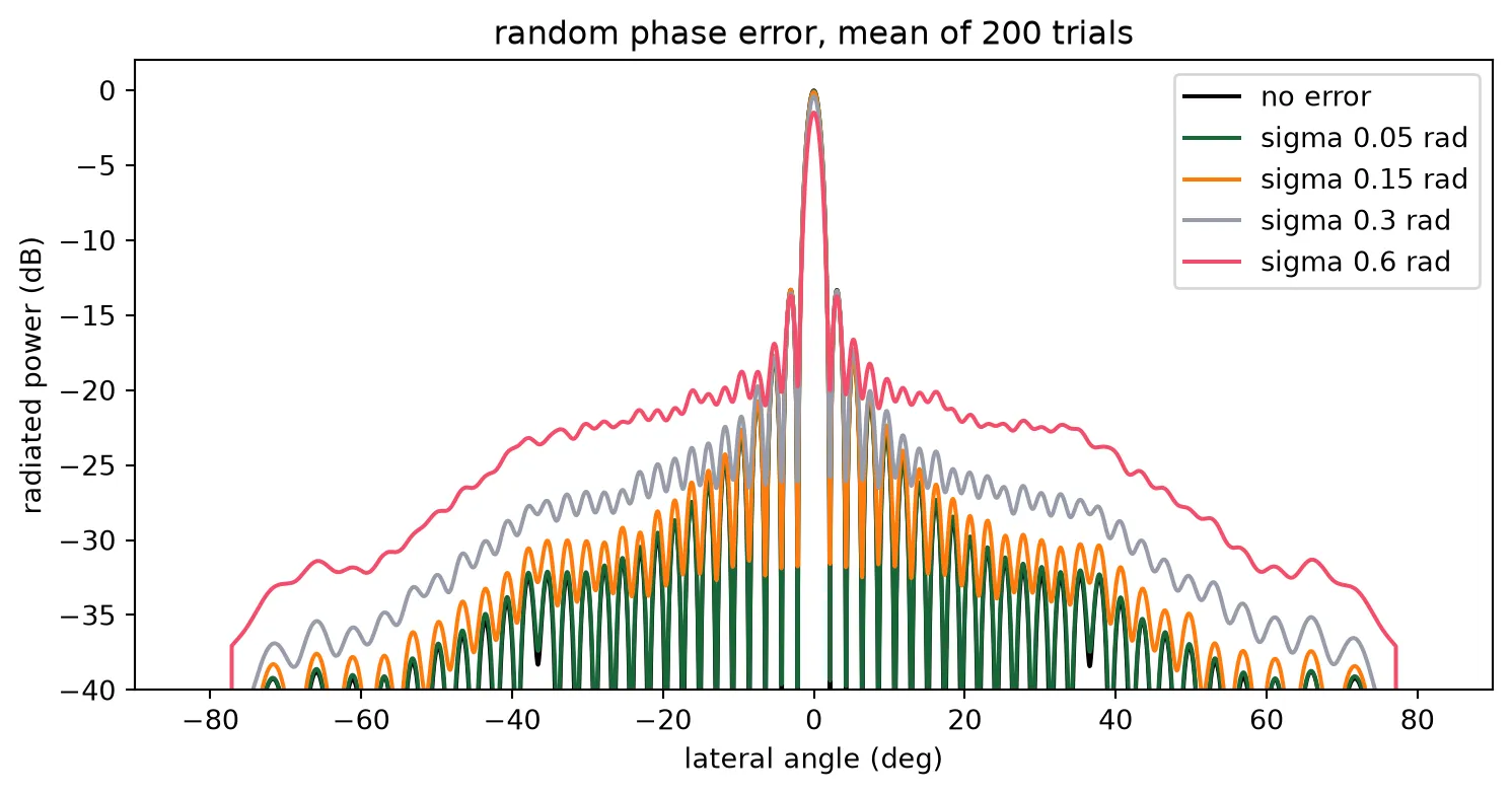

an 8-bit drive over one turn sets the phase to 0.025 rad, a 0.007 rad residual

The peak loses $\sigma^2$ in natural units, which is what the table shows: a tenth of a decibel at 0.15 rad and one and a half decibels at 0.6 rad. The lost power goes into a floor of sidelobes at roughly $\sigma^2/N$, which is what a LiDAR receiver sees as returns from directions it did not point at. An eight-bit heater drive holds the residual well under a tenth of a radian, so the floor stays below the 13 dB sidelobes the uniform aperture has anyway.

The heater

The heaters turn the phases above into electrical power, and a heat solve of the phase-shifter cross-section gives the conversion. A 200 um heater is long compared with its cross-section, so the section is solved in two dimensions: the strip, the TiN heater 0.8 um above it, the oxide, and the silicon die down to a heat sink at its back. Nothing is drawn again for this: the phase shifter of the component library is placed once or twice in a cell, the cell is extruded with the multiphysics half of every material through Component.extrude, and the technology’s blanket rules supply the wafer and the air along with the core and the heater. A floor-plan rectangle sets how far the cell, and with it the wafer, extends either side. Four steady solves and one transient are submitted together: one heater alone, for the temperature rise per milliwatt; pairs at the layout pitch and at two and three times it, for the crosstalk between channels; and a step of power on one heater, for the time constant. One milliwatt goes into the driven heater in each.

# Heater section and die, from the technology
z_heater = (
    tech.parametric_kwargs["core_thickness"]
    + tech.parametric_kwargs["heater_separation"]
)
h_heater = tech.parametric_kwargs["heater_thickness"]
clad_top = (
    z_heater
    + h_heater
    + tech.parametric_kwargs["metal_separation"]
    + tech.parametric_kwargs["metal_thickness"]
    + 1.0
)
z_wg = tech.parametric_kwargs["core_thickness"] / 2  # mid core, where the mode is
h_box = tech.parametric_kwargs["box_thickness"]  # Buried oxide (um)
die_thickness = 200.0  # Back-ground die, which sets how far the heat spreads (um)
# Oxide either side of the section, so the side walls are far from the pair (um)
lateral_pad = 400.0
air_margin = 2.0  # Air above the cladding, so the top boundary lands in the air (um)
p_probe = 1.0e-3  # Power into the driven heater (W)
w_heater = ps.parametric_kwargs["heater_width"]
l_heater = ps.parametric_kwargs["length"]

def heater_section(pitch=None, transient=None):
    """2D cross-section of one heater, or two at a pitch with only the first driven."""
    offsets = (0.0,) if pitch is None else (0.0, pitch)
    y0, y1 = -lateral_pad, (pitch or 0.0) + lateral_pad

    # The drawn phase shifter at each offset, its middle on the cut plane so the vias at its ends
    # stay out of the section, inside a floor plan as wide as the heat domain for the blanket rules
    section = pf.Component("heater_section")
    for dy in offsets:
        section.add_reference(ps).translate((-l_heater / 2, dy))
    section.add("FloorPlan", pf.Rectangle((-1, y0), (1, y1)))

    # Extrude with the multiphysics media. The heaters are named for the source and the wafer for
    # the mesh; the wafer is cut to the die thickness, since the rule runs to minus infinity.
    structures, heaters = [], []
    for solid in section.extrude(classification="electrical"):
        st = solid.to_tidy3d()
        if st.medium.name == "TiN":
            heaters.append(st)
        elif st.medium.name == "Si" and st.geometry.bounds[0][2] < -h_box - 1:
            structures.append(
                td.Structure(
                    geometry=td.Box.from_bounds(
                        (-1, y0, -h_box - die_thickness), (1, y1, -h_box)
                    ),
                    medium=st.medium,
                    name="wafer",
                )
            )
        else:
            structures.append(st)
    heaters.sort(key=lambda st: st.geometry.center[1])
    structures += [st.updated_copy(name=f"heater{k}") for k, st in enumerate(heaters)]

    # Domain: the die below, air above; the sink is the back of the die
    z0, z1 = -h_box - die_thickness, clad_top + air_margin

    # HeatSource takes a volumetric rate, so the power is spread over the heater volume
    rate = p_probe / (w_heater * h_heater * l_heater)

    # Refine around each heater, where the gradients are
    refinement = [
        td.GridRefinementRegion(
            center=(0, dy, 0.5 * (z_heater - h_box)),
            size=(0, 30.0, 2 * h_box + z_heater + 4),
            dl_internal=0.3,
            transition_thickness=10.0,
        )
        for dy in offsets
    ]

    # A transient run steps the temperature from ambient after the power switches on
    analysis = {}
    if transient is not None:
        analysis["analysis_spec"] = td.UnsteadyHeatAnalysis(
            initial_temperature=300,
            unsteady_spec=td.UnsteadySpec(
                time_step=transient["dt"], total_time_steps=transient["steps"]
            ),
        )

    return td.HeatChargeSimulation(
        center=(0, (y0 + y1) / 2, (z0 + z1) / 2),
        size=(0, y1 - y0, z1 - z0),
        # Air is the technology's background: the rules fill the die and the oxide, and the air
        # above the cladding is what no rule fills
        structures=structures,
        medium=air["electrical"],
        sources=[td.HeatSource(structures=["heater0"], rate=rate)],
        boundary_spec=[
            # Convection to the air above; the sink is the back of the die, on the domain floor
            td.HeatBoundarySpec(
                placement=td.MediumMediumInterface(mediums=["Air", "SiO2"]),
                condition=td.ConvectionBC(
                    ambient_temperature=300, transfer_coeff=10e-12
                ),
            ),
            td.HeatBoundarySpec(
                placement=td.SimulationBoundary(surfaces=["z-"]),
                condition=td.TemperatureBC(temperature=300),
            ),
        ],
        # Temperature along the waveguide plane, which is where the mode reads it
        monitors=[
            td.TemperatureMonitor(
                size=(0, td.inf, 0),
                center=(0, 0, z_wg),
                name="wg_line",
                unstructured=True,
            )
        ],
        grid_spec=td.DistanceUnstructuredGrid(
            dl_interface=h_heater / 2,
            dl_bulk=25.0,
            distance_interface=h_heater,
            distance_bulk=h_box + 2,
            non_refined_structures=["wafer"],
            mesh_refinements=refinement,
            relative_min_dl=0.5 * (h_heater / 2) / max(y1 - y0, z1 - z0),
        ),
        **analysis,
    )

# The five solves, submitted as one batch so they run side by side
pitches = (pitch_ps, 2 * pitch_ps, 3 * pitch_ps)
sims = {"one": heater_section()}
sims.update({f"pair{int(p)}": heater_section(p) for p in pitches})
# 1 us steps over 150 us
sims["step"] = heater_section(transient={"dt": 1.0e-6, "steps": 150})
batch = web.Batch(
    simulations={f"lidar_heat_{k}": s for k, s in sims.items()}, verbose=False
)
heat = batch.run(path_dir="heat_data")
print("solved:", list(sims))

solved: ['one', 'pair25', 'pair50', 'pair75', 'step']

def rise_along(name):
    """Temperature rise above ambient along the waveguide plane, and its y axis."""
    t = heat[f"lidar_heat_{name}"]["wg_line"].temperature.squeeze(drop=True) - 300.0
    return t.coords["y"].values, t.values

def rise_at(name, y_centre):
    """Mean rise over one waveguide core at y_centre."""
    y, t = rise_along(name)
    return float(t[np.abs(y - y_centre) < w_core / 2].mean())

# Thermal impedance of one heater, and what a pi shift costs
k_thermal = rise_at("one", 0.0) / (p_probe * 1e3)
dt_pi = lda0 / (2 * l_heater * dn_dt)
p_pi = dt_pi / k_thermal
r_heater = l_heater / (tin_conductivity * w_heater * h_heater)
print(
    f"thermal impedance {k_thermal:.2f} K/mW; pi needs {dt_pi:.1f} K = {p_pi:.1f} mW = {np.sqrt(p_pi * 1e-3 * r_heater):.1f} V"
)

# Crosstalk: the neighbour's rise as a fraction of the driven one's, against pitch
coupling = np.array(
    [rise_at(f"pair{int(p)}", p) / rise_at(f"pair{int(p)}", 0.0) for p in pitches]
)
for p, c in zip(pitches, coupling):
    print(f"pitch {p:3.0f} um: neighbour sees {c * 100:.1f} percent of the driven rise")

# Temperature profile across the pair at the layout pitch
y, t = rise_along(f"pair{int(pitch_ps)}")
fig, ax = plt.subplots(1, 1, figsize=(7, 4))
ax.plot(y, t)
ax.set_xlim(-60, pitch_ps + 60)
ax.set_xlabel("position across the bank (um)")
ax.set_ylabel("temperature rise in the waveguide plane (K/mW)")
ax.set_title(f"one heater driven, its neighbour {pitch_ps:.0f} um away")
plt.show()

thermal impedance 1.08 K/mW; pi needs 21.5 K = 20.0 mW = 3.8 V
pitch  25 um: neighbour sees 2.3 percent of the driven rise
pitch  50 um: neighbour sees 1.5 percent of the driven rise
pitch  75 um: neighbour sees 0.3 percent of the driven rise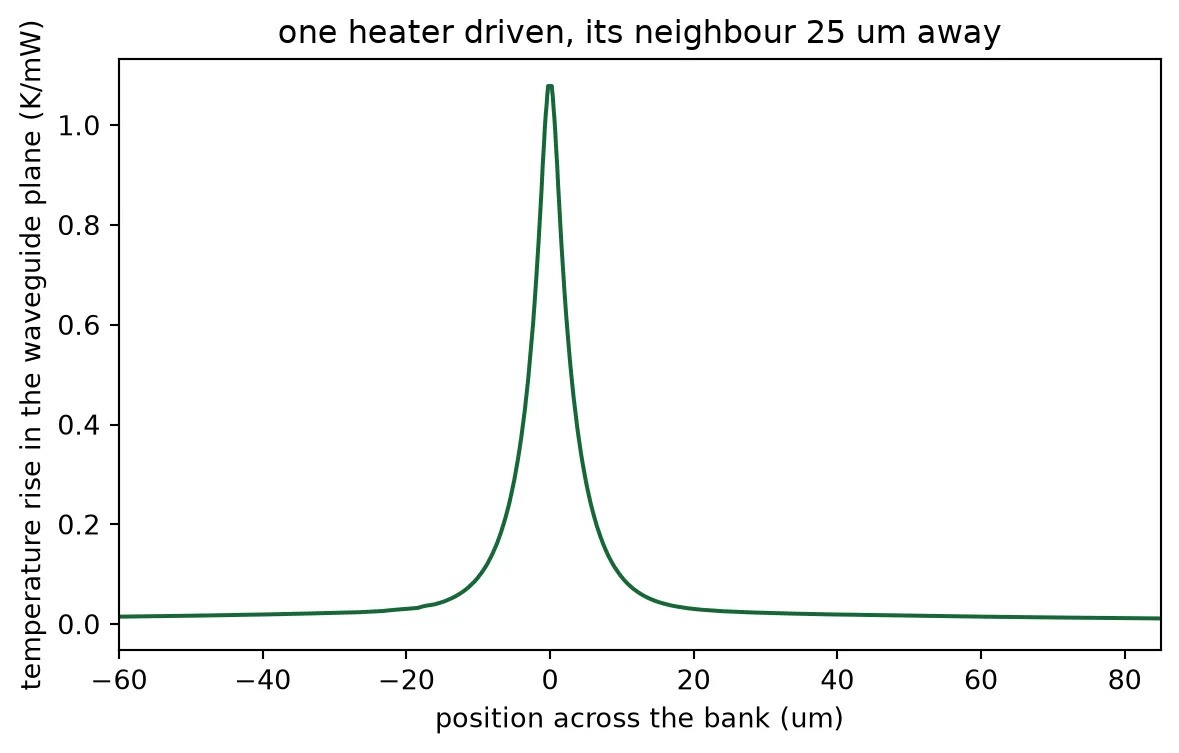

The crosstalk falls slowly with distance, because the heat spreads through the silicon die below and not only through the oxide beside the heater. A few percent from each neighbour is not negligible against a phase set to a few hundredths of a radian. It is linear, so it is corrected by construction: the temperature of every channel is the thermal coupling matrix times the vector of heater powers, and inverting that matrix gives the powers that produce the temperatures the phases ask for. The matrix is built from the three pair solves, with the coupling beyond three pitches continued along the trend they set.

# Coupling against distance: a power law through the three pairs, continued beyond them
fit = np.polyfit(np.log(pitches), np.log(coupling), 1)
distance = np.abs(np.subtract.outer(np.arange(n_ch), np.arange(n_ch))) * pitch_ps
with np.errstate(divide="ignore"):
    coupling_matrix = np.where(distance > 0, np.exp(fit[1]) * distance ** fit[0], 1.0)
print(
    f"coupling falls as distance^{fit[0]:.2f}; a channel's neighbours together add "
    f"{(coupling_matrix[n_ch // 2].sum() - 1) * 100:.0f} percent of its own rise when all heaters run alike"
)

# Powers for one steering setting, with and without the correction
phi = heater_phases(15.0)
p_target = phi / np.pi * p_pi  # mW per channel, from the phase each needs
p_corrected = np.linalg.solve(coupling_matrix, p_target)
print(
    f"steering to 15 deg: {p_target.sum():.0f} mW uncorrected, {p_corrected.sum():.0f} mW corrected, "
    f"largest single correction {np.abs(p_corrected - p_target).max():.1f} mW"
)

coupling falls as distance^-1.87; a channel's neighbours together add 10 percent of its own rise when all heaters run alike
steering to 15 deg: 581 mW uncorrected, 532 mW corrected, largest single correction 2.3 mW

Time constant and steering rate

A heater is slow. Its power is set in nanoseconds and the temperature of the waveguide follows over microseconds, first through the oxide between the two and then, more slowly, as the whole neighbourhood warms towards its steady state. The transient solve steps that response. It is not a single exponential, so two times are read off it: the time to 63 percent, which is the time constant of the fast part, and the time to 90 percent, which is when the beam has settled well enough to range with and is what sets the steering rate.

# Mean rise over the driven core at every time step
step = heat["lidar_heat_step"]["wg_line"].temperature.squeeze(drop=True)
core = step.sel(y=slice(-w_core / 2, w_core / 2)).mean("y") - 300.0
t_step = core.coords["t"].values
rise = core.values

# Time to 63 percent of the steady rise, and to 90 percent, which counts as settled here
final = rise_at("one", 0.0)
tau = t_step[np.argmax(rise >= (1 - np.exp(-1)) * final)]
t_settle = t_step[np.argmax(rise >= 0.9 * final)]
t_chirp = 10e-6  # One chirp of the ranging waveform (s), from the system budget
points_per_s = 1 / (t_settle + t_chirp)
print(
    f"63 percent in {tau * 1e6:.0f} us, 90 percent in {t_settle * 1e6:.0f} us; "
    f"one range measurement per {(t_settle + t_chirp) * 1e6:.0f} us, {points_per_s * 1e-3:.0f} thousand points per second"
)

fig, ax = plt.subplots(1, 1, figsize=(7, 4))
ax.plot(t_step * 1e6, rise / final)
for level in (1 - np.exp(-1), 0.9):
    ax.axhline(level, color="gray", linestyle="--", linewidth=1)
ax.set_xlabel("time after the power step (us)")
ax.set_ylabel("rise, fraction of the steady value")
ax.set_title("heater step response at the waveguide")
plt.show()

63 percent in 7 us, 90 percent in 24 us; one range measurement per 34 us, 29 thousand points per second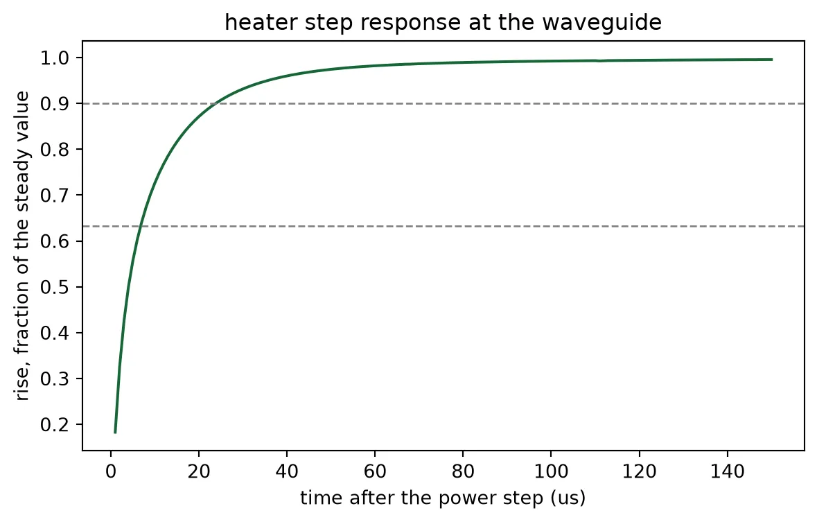

Power budget

A heater set to a phase $\varphi$ draws $\varphi / \pi$ times $P_\pi$. Over a scan every phase between zero and one turn occurs equally, so a channel draws $P_\pi$ on average and an array of 32 draws about 32 times that, with the receive array drawing the same again. The table below is that budget for the steering settings of the field of view, corrected for the thermal crosstalk, together with the rate the thermal time constant allows.

# Corrected heater powers for every angle in the table at the design wavelength
powers = np.array(
    [
        np.linalg.solve(coupling_matrix, heater_phases(t) / np.pi * p_pi)
        for t in table_angles
    ]
)
per_array = powers.sum(axis=1)
print(f"{'quantity':40s} value")
print(f"{'pi shift, one heater':40s} {p_pi:.1f} mW")
print(
    f"{'one array, average over the field of view':40s} {per_array.mean():.0f} mW ({per_array.min():.0f} to {per_array.max():.0f})"
)
print(f"{'both arrays':40s} {2 * per_array.mean():.0f} mW")
print(
    f"{'time to 63 percent, to 90 percent':40s} {tau * 1e6:.0f} us, {t_settle * 1e6:.0f} us"
)
print(f"{'range measurements per second':40s} {points_per_s * 1e-3:.0f} thousand")
print(
    f"{'heater energy per range measurement':40s} {2 * per_array.mean() * 1e-3 * (t_settle + t_chirp) * 1e6:.1f} uJ"
)

# Save everything the ranging page drives the chip with
np.savez(
    "steering_table.npz",
    angles=table_angles,
    wavelengths=wavelengths,
    phases=phase_table,
    powers_mw=powers,
    a_built=a_built,
    y_ant=y_ant,
    coupling_matrix=coupling_matrix,
    k_thermal=k_thermal,
    p_pi=p_pi,
    tau=tau,
    fov=fov,
)

quantity                                 value
pi shift, one heater                     20.0 mW
one array, average over the field of view 579 mW (459 to 678)
both arrays                              1158 mW
time to 63 percent, to 90 percent        7 us, 24 us
range measurements per second            29 thousand
heater energy per range measurement      39.4 uJ

The heaters dominate the chip’s power: two arrays of 32 at a pi each is over a watt, which is where thermo-optic phased arrays stand in the literature too. Undercutting the oxide below the heaters or thinning the die would lower it, at the cost of a slower heater and more crosstalk respectively.

Fabrication sensitivity

Three dimensions decide where the beam goes and how much light gets into it, and a process holds none of them exactly. The antenna teeth set the radiation strength, and the antenna page measured how it scales with their extent along the antenna. The strip’s width and thickness set its index, and with it the emission angle through the grating equation. The technology is parametric, so the last two are re-solved here at a five nanometre step, without redrawing anything.

# Radiated fraction over the antenna length against the tooth's extent along the antenna, from the
# measured power law in the duty cycle: a 10 nm mask bias on the tooth
extents = np.array([l_tooth_chosen - 0.01, l_tooth_chosen, l_tooth_chosen + 0.01])
alpha_at = antenna["alpha"] * (extents / l_tooth_chosen) ** duty_exponent
radiated = 1 - np.exp(-2 * alpha_at * l_antenna)
for t, r in zip(extents, radiated):
    print(
        f"tooth {t * 1e3:.0f} nm along the antenna: {r * 100:.0f} percent of the light radiated over {l_antenna:.0f} um"
    )

# Emission angle against core thickness and width: rebuild the technology, re-solve the strip
variants = {
    "nominal": {},
    "thickness +5 nm": {"core_thickness": 0.225},
    "width +5 nm": {"core_width": 0.505},
}
angle_at = {}
for name, kwargs in variants.items():
    pf.config.default_technology = lidar_soi(**kwargs)
    modes = pf.port_modes("TE_1550_500", [f0], show_progress=False, verbose=False)
    n_var = float(np.real(modes.data.n_eff.values.ravel()[0]))
    # The grating index moves with the strip index, so the angle follows the grating equation
    angle_at[name] = np.degrees(
        np.arcsin(n_avg_chosen + (n_var - n_eff_strip) - lda0 / period_chosen)
    )
pf.config.default_technology = tech
for name, angle in angle_at.items():
    print(
        f"{name:16s}: emission at {angle:.2f} deg"
        + (
            ""
            if name == "nominal"
            else f", {(angle - angle_at['nominal']) / 5 * 1e3:+.0f} millidegrees per nanometre"
        )
    )
print(f"longitudinal beam width for comparison: {np.degrees(lda0 / l_antenna):.2f} deg")

tooth 179 nm along the antenna: 91 percent of the light radiated over 1050 um
tooth 189 nm along the antenna: 92 percent of the light radiated over 1050 um
tooth 199 nm along the antenna: 93 percent of the light radiated over 1050 um
nominal         : emission at 10.00 deg
thickness +5 nm : emission at 11.08 deg, +216 millidegrees per nanometre
width +5 nm     : emission at 10.45 deg, +91 millidegrees per nanometre
longitudinal beam width for comparison: 0.08 deg

The angle sensitivities are the numbers a calibration has to absorb: a few nanometres of thickness variation across a wafer moves the emission angle by more than a beam width, so the wavelength axis of a fabricated chip is calibrated against a reference target before it is used, the same way the phase axis is. The tooth is more forgiving, since the antenna length was chosen to radiate 90 percent and a weaker grating still radiates most of the light.

What comes next

The chip can now be pointed. The ranging page takes the heater table saved above, drives the assembled chip with a chirped laser, places targets at ranges and angles, and reads range and speed out of the beat on the balanced photodiodes.