Eight-Channel DWDM Filter on Thin-Film Lithium Niobate

Download notebook (.zip)

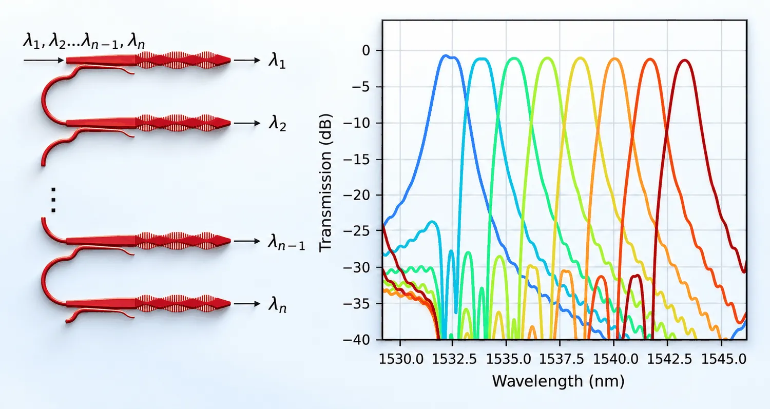
Dense wavelength-division multiplexing (DWDM) carries many channels on one waveguide, spaced a few nanometres apart in the C band. Thin-film lithium niobate (TFLN) is an attractive platform for it, because the same layer that carries the filters also carries high-speed modulators. The filter is the hard part: a shallow-etched TFLN ridge has a weak index contrast, so ring-based filters come out large and thermally sensitive.

This example builds an eight-channel DWDM demultiplexer from multimode waveguide grating (MWG) filters. A corrugation on the sidewalls of a two-mode waveguide reflects the forward TE₀ mode into the backward TE₁ mode. Because the rejected light returns in a different mode, a mode demultiplexer separates it from the incoming light, so the filter needs no circulator and no directional coupler. Three gratings in series enclose two coupled cavities, which turns the broad grating reflection into one narrow flat-top passband. The wavelength of a whole stage is then set by a single number: the length $L_t$ of the phase section between gratings.

The notebook covers:

• the LNOI layer stack and the two-mode waveguide the grating works with,
• the cavity split into gratings and phase sections, so the channels come almost free,
• the linear relation between $L_t$ and channel wavelength, measured with a three-point sweep,
• the mode demultiplexer and the width transitions, each with its own model,
• the eight-stage cascade and its circuit response.

Reference

1. Zhu, Mingyu, et al. “Multichannel Lithium-Niobate-On-Insulator Photonic Filter for Dense Wavelength-Division Multiplexing.” ACS Photonics 2025 12 (2), 588-596, doi: 10.1021/acsphotonics.4c00884.

Note on cost: the two grating simulations come to 6.5 FlexCredits together and are reused at every channel, so the channel count does not drive the bill. The mode demultiplexer is the largest single run in the notebook. The three width transitions use eigenmode expansion and are negligible. Every result is cached, so re-running the notebook afterwards is free.

For more integrated photonic examples, please visit our examples page. If you are new to the finite-difference time-domain (FDTD) method, we highly recommend going through our FDTD101 tutorials.

import time

import matplotlib.pyplot as plt
import numpy as np
import photonforge as pf
import tidy3d as td
from photonforge.live_viewer import LiveViewer

# Browser-based layout viewer; every component built below is sent to it.
viewer = LiveViewer()

LiveViewer started at http://127.0.0.1:45127. Call its 'stop()' method to free the port.

The LNOI platform

The stack is x-cut TFLN: a 400 nm film with a 200 nm partial etch, so a 200 nm slab remains everywhere outside the ridge, air above and buried oxide below. The etch leaves 60 degree sidewalls, measured from the wafer surface, which matters for a corrugated grating and is modelled explicitly rather than as a vertical wall.

Only the media come from Tidy3D. Every geometry, model, and circuit object below is PhotonForge.

lda0 = 1.540                                            # Centre wavelength of the channel comb (um)
ldas = np.linspace(1.525, 1.555, 401)                   # Fine grid across the eight channels
freqs = pf.C_0 / ldas
lam = ldas * 1e3                                        # The same grid in nm, for every plot below
freqs_coarse = pf.C_0 / np.linspace(1.520, 1.560, 21)   # Coarse grid for the smooth components

n_o, n_e = 2.211, 2.138       # Ordinary and extraordinary indices of x-cut LN at 1.55 um
n_sio2 = 1.444                # Buried oxide index
h_film, h_slab = 0.400, 0.200                           # Film thickness and remaining slab (um)
sidewall_deg = 30.0           # Measured from the wafer normal, so 60 degree sidewalls
ridge_layer = (1, 0)          # GDS layer of the unetched ridge

The film is birefringent, so it is described with an AnisotropicMedium. Light propagates along $x$ and the extraordinary axis lies in the plane of the wafer, transverse to propagation, so the extraordinary index goes on the $yy$ component.

A PhotonForge Technology bundles the layer stack with the port specifications, so every component built afterwards inherits the same cross sections and mode solver settings. Four cross sections are needed: the 1.85 µm multimode waveguide that the grating is written on, the 2.0 µm end of the mode demultiplexer, its 1.0 µm single-mode input, and the 0.6 µm routing waveguide. The ridge extrusion carries sidewall_angle referenced to the top of the film, which puts the slope on every edge including the grating tooth faces.

Each specification takes its modes in order of effective index and applies no polarization filter. On this ridge the ordering already puts TE₀ and TE₁ first, with the nearest TM mode about 0.07 lower in index, so a filter would change nothing. It is worth leaving out: a filtered specification forces the solver to store the full mode field profile at every frequency so that it can re-map mode order, which turns a result of a few hundred kilobytes into several gigabytes.

# Anisotropic LN, with the extraordinary axis transverse to propagation.
ln = td.AnisotropicMedium(
    xx=td.Medium(permittivity=n_o**2),
    yy=td.Medium(permittivity=n_e**2),
    zz=td.Medium(permittivity=n_o**2),
    name="LN_xcut",
)
sio2 = td.Medium(permittivity=n_sio2**2, name="SiO2")
air = td.Medium(permittivity=1.0, name="air")

# Mode solver window: 1.2 um below the film and 1.6 um above it.
port_limits = (-1.2, 1.6)

# One LayerSpec: everything drawn on it stays unetched and becomes the ridge.
layers = {"RIDGE": pf.LayerSpec(ridge_layer, "Unetched LN ridge (400 nm)", "#c0002018", "/")}

# Buried oxide, then the slab that survives the partial etch, then the sloped ridge on top.
extrusion_specs = [
    pf.ExtrusionSpec(pf.MaskSpec(), sio2, (-pf.Z_INF, 0.0)),
    pf.ExtrusionSpec(pf.MaskSpec(), ln, (0.0, h_slab)),
    pf.ExtrusionSpec(
        pf.MaskSpec(ridge_layer), ln, (h_slab, h_film),
        sidewall_angle=sidewall_deg, reference="top",
    ),
]

# The four waveguide cross sections used in the design. Modes are taken in order of effective
# index, which on this ridge already puts TE0 and TE1 first, so no polarization filter is needed.
ports = {
    "MM_1850": pf.PortSpec("Grating waveguide, TE0 and TE1", 5.5, port_limits, num_modes=2,
                           target_neff=1.82,
                           path_profiles=[(1.850, 0, ridge_layer)], default_radius=100.0),
    "MM_2000": pf.PortSpec("Mode demultiplexer wide end, TE0 and TE1", 5.5, port_limits, num_modes=2,
                           target_neff=1.82,
                           path_profiles=[(2.000, 0, ridge_layer)], default_radius=100.0),
    "SM_1000": pf.PortSpec("Mode demultiplexer input, TE0", 4.5, port_limits, num_modes=1,
                           target_neff=1.80,
                           path_profiles=[(1.000, 0, ridge_layer)], default_radius=100.0),
    "SM_600": pf.PortSpec("Single-mode routing waveguide, TE0", 4.0, port_limits, num_modes=1,
                          target_neff=1.75,
                          path_profiles=[(0.600, 0, ridge_layer)], default_radius=100.0),
}

# Make this the default technology so components do not have to name it.
tech = pf.Technology("LNOI 400/200 nm, 60 degree sidewalls", "1.0", layers, extrusion_specs, ports, air)
pf.config.default_technology = tech

The whole design rests on the 1.85 µm waveguide supporting exactly two TE modes with well separated effective indices, because the grating couples one into the other. Solving the port modes gives those indices and shows the cross section that the sloped sidewall produces.

# Solve the two TE modes of the grating waveguide at the centre wavelength.
modes = pf.port_modes("MM_1850", [pf.C_0 / lda0], verbose=False)
n_eff = modes.data.n_eff.values.real.ravel()
print(f"n_eff at {lda0} um: TE0 = {n_eff[0]:.4f}, TE1 = {n_eff[1]:.4f}")

fig, axs = plt.subplots(1, 3, figsize=(13, 3), tight_layout=True)

# Left panel: the ridge cross section as the mode solver sees it.
pf.tidy3d_plot(tech.ports["MM_1850"], ax=axs[0])
axs[0].set_title("MM_1850 cross section")

# Right panels: the even TE0 and odd TE1 field profiles the grating couples.
for i, ax in enumerate(axs[1:]):
    modes.plot_field("Ey", val="abs", mode_index=i, ax=ax, cmap="magma", eps_alpha=0.0)
    ax.set_title(f"TE$_{i}$, $n_{{eff}}$ = {n_eff[i]:.4f}")
plt.show()

n_eff at 1.54 um: TE0 = 1.8112, TE1 = 1.7281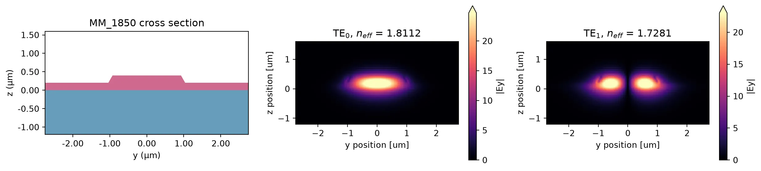

How the filter works

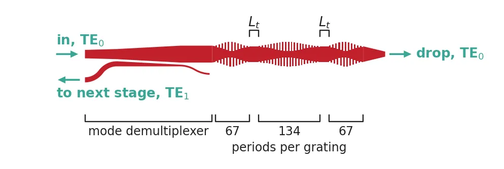
One stage of the demultiplexer, with the phase sections drawn longer than they are so that the three gratings separate visually.

The grating couples forward TE₀ to backward TE₁

A grating couples two modes when its grating vector makes up the mismatch between their propagation constants. Here one mode travels forward and the other backward, so their propagation constants have opposite signs and the mismatch is their sum:

$$\Lambda = \frac{\lambda}{n_{\mathrm{TE}_0} + n_{\mathrm{TE}_1}}$$

With the indices solved above this is about 435 nm at 1.54 µm, and the design uses $\Lambda = 433.3$ nm.

Phase matching alone is not enough: the perturbation also has to have the right symmetry. TE₀ is even about the waveguide centre line and TE₁ is odd, so a perturbation that is even about that line, such as a uniform width modulation, gives zero overlap between them. The corrugation used here is antisymmetric instead. The waveguide keeps a constant width of 1.85 µm while its centre line steps by $+\delta/2$ for half a period and by $-\delta/2$ for the other half, so the teeth on the two sidewalls are offset by $\Lambda/2$. That perturbation is odd about the centre line, which is exactly what couples an even mode to an odd one.

Why the tooth depth follows three Gaussian humps

A grating that starts and stops abruptly has a rectangular coupling envelope, and its reflection spectrum carries the side lobes that go with it. The corrugation depth here is apodized instead,

$$\delta_i = \delta \, \exp\left[-b\,\frac{(i - N/2)^2}{N^2}\right], \qquad b = 10$$

so the coupling ramps up and fades away over each grating. The side lobes drop and the stop-band floor sits far below the channel level, which is what keeps crosstalk between neighbouring channels low.

The depth profile of one cavity therefore shows three Gaussian humps, one per grating, not one. The three humps are three mirrors, and their lengths are 67, 134, and 67 periods.

Why three mirrors instead of two

A single grating is a mirror: inside its stop band it returns TE₀ as backward TE₁ over a band many nanometres wide, far too broad for a DWDM channel. Two gratings enclose one Fabry-Perot cavity, which transmits a narrow Lorentzian line at each resonance. Three gratings enclose two cavities, coupled to each other through the middle mirror. Two coupled resonances sit side by side, and when their separation is comparable to their linewidth the pair merges into a single passband with a flat top and steeper edges than one resonance can give. The middle grating is twice as long as the outer two, so it is the stronger mirror: the coupling between the two cavities is weaker than the coupling to the outside world, which is the ordering a bandpass filter needs.

How one stage drops a channel and passes the rest

Light enters a stage as TE₀. Two things then happen at once:

• At the cavity resonance, the light tunnels through all three mirrors and leaves the far end of the cavity as forward TE₀. This is the channel that the stage drops.
• Everywhere else in the stop band, the gratings reflect it, and it comes back to the input end as backward TE₁. This is everything the stage does not drop.

The rejected light is in a different mode from the incoming light, so it can be separated by geometry alone. The mode demultiplexer placed in front of the cavity carries forward TE₀ from its single-mode input into the multimode waveguide, and pulls backward TE₁ coming out of the multimode waveguide into a separate narrow waveguide. That narrow waveguide feeds the next stage. Nothing in this path is a circulator or a directional coupler, which is the reason for working in reflection between two modes in the first place.

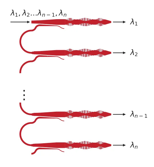
Eight stages in series, each with a slightly different phase-section length $L_t$, therefore take one channel each out of the comb and pass the remainder along. The hairpin between stages is the route that carries the rejected light from one through port to the next input.

The cavity, one grating at a time

The cavity is three gratings separated by two phase sections. Only the phase sections change from channel to channel, so simulating the whole cavity again for every channel repeats the expensive part for nothing. Each grating is instead simulated once on its own, and the cavity is assembled from those results with the phase sections carrying the only thing that differs.

This works because the corrugation is apodized. At the ends of a grating the teeth are about 100 nm deep on a 1850 nm waveguide, so the joints sit in waveguide that is almost unperturbed, where the two guided modes describe the field well.

A grating is built the way the whole cavity would be: the segment list walks along $x$ accumulating the length and centre-line offset of each piece, and the two sidewalls are read off that list. A short stub at each end puts the ports on the waveguide centre line, which the last tooth would otherwise leave offset by half a tooth depth.

@pf.parametric_component
def grating(
    *,
    n_periods: int = 67,        # Number of corrugation periods
    w_mwg: float = 1.850,       # Multimode waveguide width (um)
    period: float = 0.4333,     # Corrugation period (um)
    delta: float = 1.100,       # Peak corrugation depth (um)
    duty: float = 0.5,          # Fraction of the period spent on the upper offset
    b_apod: float = 10.0,       # Gaussian apodization strength
    pad: float = 0.1,           # On-axis stub at each end, so the ports sit on the centre line
) -> pf.Component:
    """One Gaussian-apodized multimode waveguide grating."""

    # Gaussian apodization of the tooth depth across the grating.
    i = np.arange(1, n_periods + 1)
    depths = delta * np.exp(-b_apod * (i - n_periods / 2) ** 2 / n_periods**2)

    # Each period steps the centre line up then down, offsetting the two sidewalls by half a period.
    segments = [(pad, 0.0)]
    for d in depths:
        segments += [(period * duty, 0.5 * d), (period * (1 - duty), -0.5 * d)]
    segments.append((pad, 0.0))

    # Turn the segment list into the two sidewalls of a constant-width waveguide.
    x, top, bottom = 0.0, [], []
    for length, offset in segments:
        top += [(x, offset + 0.5 * w_mwg), (x + length, offset + 0.5 * w_mwg)]
        bottom += [(x, offset - 0.5 * w_mwg), (x + length, offset - 0.5 * w_mwg)]
        x += length

    # Close the outline by running back along the bottom sidewall.
    c = pf.Component(f"GRATING_{n_periods}")
    c.add("RIDGE", pf.Polygon(top + bottom[::-1]))

    # Find the two waveguide ends from the geometry and name them input first.
    p_in, p_out = sorted(c.detect_ports(["MM_1850"], on_boundary="x"), key=lambda p: p.center[0])
    c.add_port(p_in, port_name="P0")
    c.add_port(p_out, port_name="P1")

    # A lone grating does not resonate, so the default run time is long enough.
    c.add_model(pf.Tidy3DModel(verbose=False))
    return c

viewer(grating())

Plotting the tooth depths of the three gratings in sequence shows the apodization, and shows the outer gratings at half the length of the middle one.

# Read the shape back from the component, so no number is repeated here.
n_periods = (67, 134, 67)
shape = grating().parametric_kwargs

# Rebuild the apodized tooth depths of the three gratings.
depths = np.concatenate([
    shape["delta"] * np.exp(-shape["b_apod"] * (np.arange(1, n + 1) - n / 2) ** 2 / n**2)
    for n in n_periods
])

fig, ax = plt.subplots(figsize=(7.5, 2.6), tight_layout=True)
ax.plot(np.arange(depths.size) * shape["period"], depths * 1e3, color="#c0202a", lw=1.8)
ax.set(xlabel="Position along the cavity (um)", ylabel="Tooth depth (nm)")
ax.grid(alpha=0.3)
plt.show()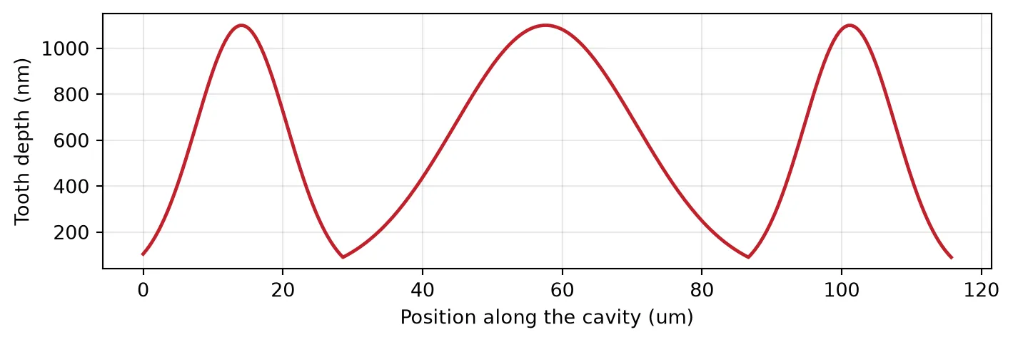

What the decomposition saves

The gratings are the only cloud simulations that would otherwise scale with the number of channels. Run once, they serve every channel. These figures were measured on this design.

	FDTD runs	billed
One whole cavity, single excitation	1	14.9 FlexCredits
Eight channels simulated that way	8	about 120 FlexCredits
Grating of 67 periods, every excitation	4	1.9 FlexCredits
Grating of 134 periods, every excitation	4	4.6 FlexCredits
Both gratings, reused at every channel	8	6.5 FlexCredits

Two effects compound. Each grating is a fraction of the cavity length, and a lone grating does not resonate, so its field decays quickly and the run stops early, while the cavity has to be followed until it rings down. Eight channels therefore cost less than half of one cavity, and every further channel is free.

Each grating needs all four excitations, because the corrugation is not mirror symmetric: a period runs up then down, which reverses when the grating is read from the other end.

# The only cloud simulations in the notebook. Launch both, then collect.
gratings = {n: grating(n_periods=n) for n in (67, 134)}
runners = {n: g.active_model.start(g, freqs) for n, g in gratings.items()}
while any(r.status["message"] == "running" for r in runners.values()):
    time.sleep(30)

# Store each result so the cavity reads data instead of calling a solver.
for n, g in gratings.items():
    g.add_model(pf.DataModel(runners[n].s_matrix, interpolation_method="linear"), "FDTD data")
print("gratings simulated:", sorted(gratings))

gratings simulated: [67, 134]

Assembling the cavity

The cavity is now a circuit: the two simulated gratings, the phase sections between them, and the straight leads at either end. A phase section is a plain two-mode waveguide, and straight already comes with a WaveguideModel, so no model has to be added. With no effective index set, that model solves the cross section and gives each mode the index it actually has, with no mixing between them, which is all a straight waveguide does. The reference_chain function places the pieces end to end, and the numbers in its sequence become these straight sections.

$L_t$ is still the only thing that differs between channels, but changing it now only re-assembles the circuit.

@pf.parametric_component
def mwg_cavity(
    *,
    lt: float = 0.434,                 # Phase section between gratings, the channel knob (um)
    n_periods: tuple = (67, 134, 67),  # Periods in the three gratings
    l_in: float = 1.5,                 # Straight lead into the first grating (um)
    l_out: float = 10.5,               # Straight lead out of the last grating (um)
    pad: float = 0.1,                  # Stub already carried at each grating end (um)
) -> pf.Component:
    """Third-order Fabry-Perot cavity, assembled from the simulated gratings."""

    # Lead, then each grating separated by a phase section, then the output lead. The numbers
    # in the sequence are the straight sections, with the port specification of the gratings.
    gap = f" - {lt - 2 * pad} - "
    sequence = f"{l_in - pad} - " + gap.join(f"g{n}" for n in n_periods) + f" - {l_out - pad}"
    refs = pf.reference_chain({f"g{n}": gratings[n] for n in n_periods}, sequence)

    # Chain the pieces end to end and expose the two outermost ports.
    c = pf.Component(f"MWG_CAVITY_LT{lt * 1e3:.0f}")
    c.add(*refs)
    c.add_port(refs[0]["P0"], port_name="P0")
    c.add_port(refs[-1]["P1"], port_name="P1")

    c.add_model(pf.CircuitModel(verbose=False), "Circuit")
    return c

cavity = mwg_cavity()
print(f"cavity length: {cavity.size()[0]:.3f} um")
viewer(cavity)

cavity length: 128.992 um

LayoutSchematic

The response of one cavity

Composing the circuit gives the whole two-port, two-mode S matrix at once, so both quantities of interest come from the same call: P0@0 to P1@0 is the forward TE₀ that leaves the far end, and P0@0 to P0@1 is the backward TE₁ that returns to the input.

# A local calculation: the gratings read stored data and the phase sections are analytic.
s_cavity = cavity.s_matrix(freqs)

# The drop port is forward TE0 through the cavity, the through port is backward TE1.
drop_db = 10 * np.log10(np.abs(s_cavity[("P0@0", "P1@0")]) ** 2)
through_db = 10 * np.log10(np.abs(s_cavity[("P0@0", "P0@1")]) ** 2)

fig, ax = plt.subplots(figsize=(7.5, 4.2), tight_layout=True)
ax.plot(lam, through_db, color="#1060d0", lw=2.4, label="Through port, backward TE$_1$")
ax.plot(lam, drop_db, color="#e8000b", lw=2.4, label="Drop port, forward TE$_0$")
ax.set(xlim=(lam.min(), lam.max()), ylim=(-60, 5),
       xlabel="Wavelength (nm)", ylabel="Transmission (dB)")
ax.grid(alpha=0.3)
ax.legend(loc="lower left")
plt.show()

Uploading task 'Mode-GratingwaveguideTE0andTE1…'
Starting task 'Mode-GratingwaveguideTE0andTE1': https://tidy3d.simulation.cloud/workbench?taskId=mo-3669bf08-0a5c-4bfa-9d10-286a9ea906ae
Downloading data from 'Mode-GratingwaveguideTE0andTE1'…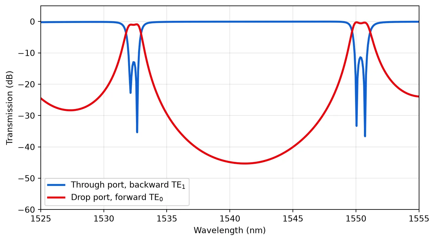

The through port sits near 0 dB right across the window, so the gratings reflect almost everything: with a corrugation this deep the stop band is wider than the 30 nm plotted here. Inside it the drop port shows a comb of narrow flat-topped passbands about 18 nm apart. That spacing is the free spectral range of the coupled cavities, and it is the budget the channel comb has to fit into.

Each passband is the channel its stage takes; everything else continues to the next stage. The design uses the branch near 1532 nm, so everything below searches a 16 nm band around it, which holds exactly one resonance of the comb for every phase-section length used here.

Setting the channel wavelength with Lₜ

Every stage uses the same gratings, so the stop band never moves. What moves is the resonance inside it, and it is set by the round-trip phase of the two cavities, which is proportional to the phase-section length $L_t$. The response is linear over the range of interest, so three points are enough to calibrate it.

Because the gratings are already simulated, each of these costs nothing but a circuit composition.

lt_sweep = [0.434, 0.564, 0.695]          # Phase section lengths to calibrate against (um)

# Re-assembling the circuit at each value is all that is needed.
s_sweep = [mwg_cavity(lt=lt).s_matrix(freqs) for lt in lt_sweep]

The resonance of each cavity is the drop-port maximum inside the design band. Restricting the search to that band is what separates the branch being designed from its neighbour in the comb, which can be the stronger of the two.

channel_band = (1530.0, 1546.0)     # Band the comb is placed in, narrower than one free spectral range
in_band = (lam > channel_band[0]) & (lam < channel_band[1])

# Each cavity resonance is the strongest drop peak inside that band.
peaks = [lam[in_band][np.argmax((np.abs(s[("P0@0", "P1@0")]) ** 2)[in_band])] for s in s_sweep]

# Straight line through the three points: this is the tuning calibration.
slope, intercept = np.polyfit(np.array(lt_sweep) * 1e3, peaks, 1)
print("resonances (nm):", np.round(peaks, 2))
print(f"tuning slope: {slope:.4f} nm of wavelength per nm of Lt")

resonances (nm): [1532.58 1537.6  1543.15]
tuning slope: 0.0405 nm of wavelength per nm of Lt

fig, axs = plt.subplots(1, 2, figsize=(12, 4), tight_layout=True)

# Left: the three measured spectra, showing the resonance sliding through a fixed stop band.
for lt, s, color in zip(lt_sweep, s_sweep, ("#1b5e20", "#e8850b", "#7030a0")):
    axs[0].plot(lam, 10 * np.log10(np.abs(s[("P0@0", "P1@0")]) ** 2),
                color=color, lw=1.8, label=f"$L_t$ = {lt * 1e3:.0f} nm")
axs[0].set(xlim=(lam.min(), lam.max()), ylim=(-60, 5),
           xlabel="Wavelength (nm)", ylabel="Drop transmission (dB)")
axs[0].grid(alpha=0.3)
axs[0].legend(loc="lower left")

# Right: the calibration line the channel grid is built from.
lt_fine = np.linspace(0.40, 0.73, 50) * 1e3
axs[1].plot(lt_fine, np.polyval([slope, intercept], lt_fine), color="#e8850b", lw=2,
            label=f"fit, {slope:.3f} nm/nm")
axs[1].plot(np.array(lt_sweep) * 1e3, peaks, "o", color="#1b5e20", ms=8, label="simulated")
axs[1].set(xlabel="$L_t$ (nm)", ylabel="Resonance wavelength (nm)")
axs[1].grid(alpha=0.3)
axs[1].legend()
plt.show()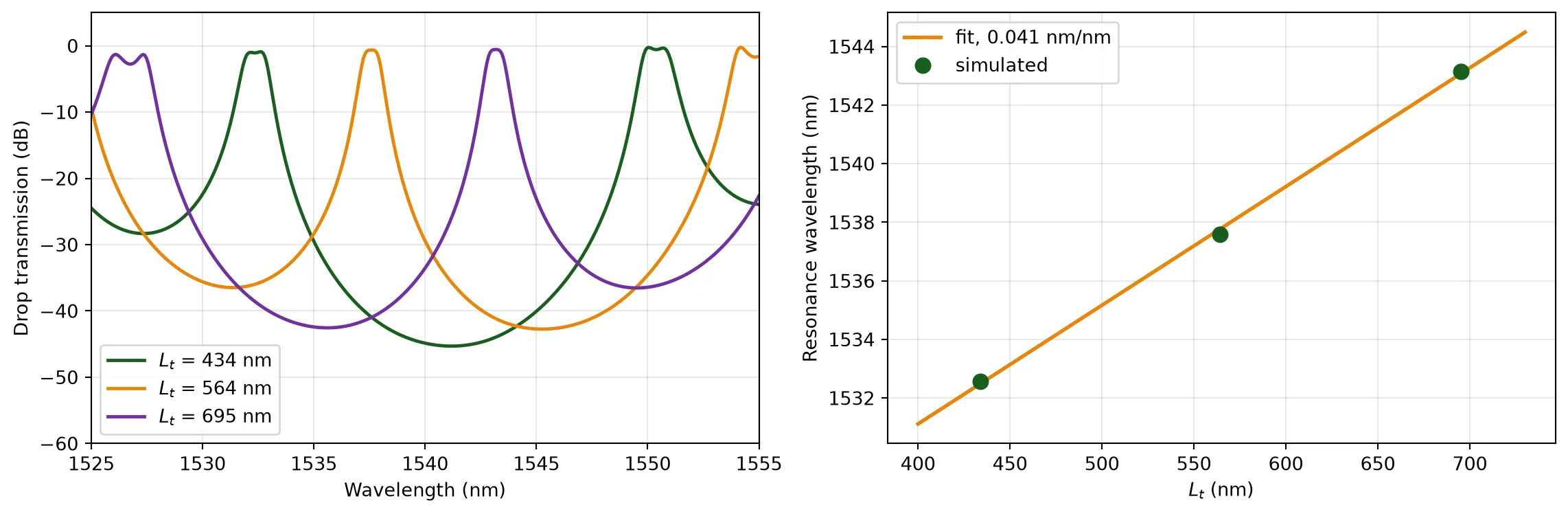

Eight channels from the calibration line

The calibration converts a target channel grid into eight phase-section lengths. Evenly spaced $L_t$ gives an evenly spaced comb, so the eight values are simply spread across the calibrated range and rounded to the nanometre layout grid.

Each cavity is a circuit over the same two gratings, so the eight of them together add nothing to the simulation budget.

# Eight evenly spaced phase sections across the calibrated range, on the 1 nm layout grid.
lt_channels = np.round(np.linspace(lt_sweep[0], lt_sweep[-1], 8), 3)
print("Lt per channel (nm):", np.round(lt_channels * 1e3, 1))
print(f"expected channel spacing: {slope * np.diff(lt_channels * 1e3)[0]:.2f} nm")

# One circuit per channel, over the gratings that are already simulated.
cavities = [mwg_cavity(lt=lt) for lt in lt_channels]

Lt per channel (nm): [434. 471. 509. 546. 583. 620. 658. 695.]
expected channel spacing: 1.50 nm

Mode demultiplexer

Each stage needs a component that pulls backward TE₁ out of the multimode waveguide without disturbing forward TE₀. An adiabatic dual-core coupler does it: a narrow waveguide runs alongside a widening multimode waveguide, and along that taper the TE₁ supermode moves into the narrow waveguide while TE₀ stays where it is.

The coupling gap is set by the etch, not by the coupling strength. The ridge is 200 nm tall with 60 degree sidewalls, so each wall flares 116 nm outward between the top of the ridge and the slab. A gap drawn at 250 nm therefore closes to 19 nm where the two ridges meet the slab, which is below what the process can hold and below what the simulation grid can resolve. Drawn at 350 nm it is still 119 nm at the base, and the transfer has more room to stay adiabatic: the wider gap gives lower conversion loss and lower crosstalk than the tighter one.

Port A is the single-mode input, C is the multimode side facing the cavity, and B is the narrow through port that feeds the next stage. Reading the device from C backwards: the narrow waveguide starts at 0.2 µm, far from phase matching, then widens to 0.6 µm while the multimode waveguide narrows from 2.0 µm to 1.0 µm, so TE₁ transfers across and emerges as TE₀ at B. The narrow waveguide ends 2 µm short of the multimode end, where it carries no power.

@pf.parametric_component
def mode_demux(
    *,
    w_in: float = 1.0,        # Single-mode input width of the wide waveguide (um)
    w_mid: float = 1.2,       # Wide waveguide width at the start of the coupling section (um)
    w_out: float = 2.0,       # Multimode width facing the cavity (um)
    w_tap1: float = 0.6,      # Narrow waveguide width at the through port (um)
    w_tap2: float = 0.2,      # Narrow waveguide width at the multimode end (um)
    l_a: float = 50.0,        # Approach section length (um)
    l_b: float = 100.0,       # Coupling section length (um)
    l_c: float = 50.0,        # Separation section length (um)
    gap_in: float = 2.25,     # Edge-to-edge gap at the input (um)
    gap_mid: float = 0.35,    # Edge-to-edge gap through the coupling section (um)
    gap_out: float = 1.25,    # Edge-to-edge gap where the narrow waveguide peels away (um)
    l_tip: float = 2.0,       # How far short of the multimode end the narrow waveguide stops (um)
) -> pf.Component:
    """Adiabatic dual-core coupler: TE1 in the wide waveguide becomes TE0 in the narrow one."""

    # The wide waveguide widens monotonically from single mode to two modes.
    x1, x2, x3 = l_a, l_a + l_b, l_a + l_b + l_c
    wide = pf.Path((0, 0), w_in).segment((x1, 0), w_mid).segment((x2, 0), w_out).segment((x3, 0))

    # Centre lines of the narrow waveguide, set by the edge-to-edge gap at each station.
    y0 = 0.5 * w_in + gap_in + 0.5 * w_tap1
    y1 = 0.5 * w_mid + gap_mid + 0.5 * w_tap1
    y2 = 0.5 * w_out + gap_mid + 0.5 * w_tap2
    y3 = 0.5 * w_out + gap_out + 0.5 * w_tap2

    # The narrow waveguide comes in, runs alongside while narrowing, then peels away and stops.
    narrow = pf.Path((0, y0), w_tap1).s_bend((x1, y1)).segment((x2, y2), w_tap2).s_bend((x3 - l_tip, y3))

    c = pf.Component("MODE_DEMUX")
    c.add("RIDGE", wide, narrow)

    # Detect the three waveguide ends; they come back in the order the specs are listed.
    port_a, port_b, port_c = c.detect_ports(["SM_1000", "SM_600", "MM_2000"], on_boundary="x")
    c.add_port(port_a, port_name="A")
    c.add_port(port_b, port_name="B")
    c.add_port(port_c, port_name="C")

    c.add_model(pf.Tidy3DModel(verbose=False))
    return c

mux = mode_demux()
viewer(mux)

This is the one component in the design whose waveguides are not straight: the narrow one follows two long shallow S-bends. Eigenmode expansion represents a device as a stack of uniform cells, so a gradual lateral offset needs a great many of them, while FDTD handles it directly. The mode demultiplexer therefore uses FDTD, and the straight transitions further down use eigenmode expansion. Only two excitations matter in the cascade, forward TE₀ at A and backward TE₁ at C. They are evaluated on the coarse frequency grid because the response is smooth, and stored as a DataModel so the circuit solve interpolates instead of re-simulating.

# Two excitations on a coarse grid are enough for a response this smooth.
s_mux = mux.s_matrix(freqs_coarse, model_kwargs={"inputs": ("A@0", "C@1")})
mux.add_model(pf.DataModel(s_mux, interpolation_method="cubicspline"), "FDTD data")

# The two wanted paths and the two crosstalk paths of the device.
lam_mux = s_mux.wavelengths * 1e3
curves = {
    "C TE$_1$ to B TE$_0$, rejected light to the next stage": np.abs(s_mux[("C@1", "B@0")]) ** 2,
    "A TE$_0$ to C TE$_0$, input into the cavity": np.abs(s_mux[("A@0", "C@0")]) ** 2,
    "C TE$_1$ to A TE$_0$, crosstalk": np.abs(s_mux[("C@1", "A@0")]) ** 2,
    "A TE$_0$ to B TE$_0$, crosstalk": np.abs(s_mux[("A@0", "B@0")]) ** 2,
}

fig, ax = plt.subplots(figsize=(7.5, 4), tight_layout=True)
for label, value in curves.items():
    ax.plot(lam_mux, 10 * np.log10(np.maximum(value, 1e-8)), lw=1.8, label=label)
ax.set(xlabel="Wavelength (nm)", ylabel="Transmission (dB)", ylim=(-50, 2))
ax.grid(alpha=0.3)
ax.legend(fontsize=8, loc="lower right")
plt.show()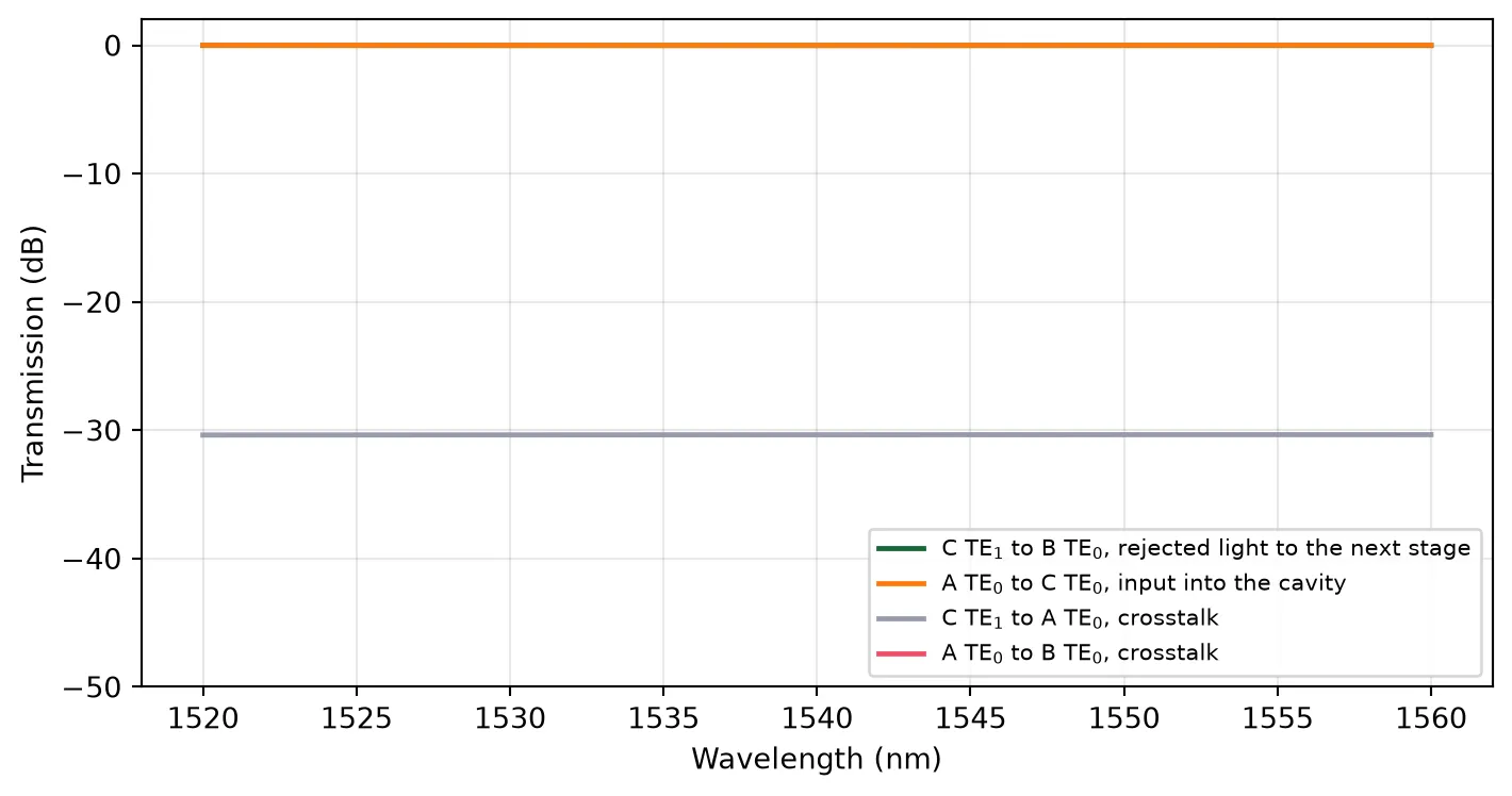

Width transitions

Three width transitions connect the pieces: the multimode end of the demultiplexer to the slightly narrower grating waveguide, the grating waveguide to the single-mode drop waveguide, and the narrow through waveguide back to the demultiplexer input. They are straight and adiabatic, which is the regime where eigenmode expansion is both accurate and far cheaper than FDTD, so they use an EMEModel. All three come out lossless at the hundredth-of-a-decibel level, so they contribute nothing to the channel budget. The cell reports the departure from unit transmission rather than a signed loss, because at that level the numerical floor of the eigenmode expansion is the larger effect.

# Uniform EME grids; longer transitions need more cells to follow the width change.
mode_spec = td.EMEModeSpec(num_modes=8)
eme = dict(grid_spec=20, verbose=False)
tapers = {
    "mux to cavity": pf.parametric.transition(
        port_spec1="MM_2000", port_spec2="MM_1850", length=5.0, name="TAPER_MUX_CAVITY",
        model=pf.EMEModel(eme_grid_spec=td.EMEUniformGrid(num_cells=12, mode_spec=mode_spec), **eme)),
    "cavity to drop": pf.parametric.transition(
        port_spec1="MM_1850", port_spec2="SM_600", length=25.0, name="TAPER_DROP",
        model=pf.EMEModel(eme_grid_spec=td.EMEUniformGrid(num_cells=30, mode_spec=mode_spec), **eme)),
    "through to mux": pf.parametric.transition(
        port_spec1="SM_600", port_spec2="SM_1000", length=15.0, name="TAPER_THROUGH",
        model=pf.EMEModel(eme_grid_spec=td.EMEUniformGrid(num_cells=15, mode_spec=mode_spec), **eme)),
}

# Run each transition once and store the result, so the circuit solve reads data instead of solving.
for label, taper in tapers.items():
    s = taper.s_matrix(freqs_coarse)
    taper.add_model(pf.DataModel(s, interpolation_method="cubicspline"), "EME data")
    # Worst departure from unit TE0 transmission across the band.
    loss = -10 * np.log10(np.abs(s[("P0@0", "P1@0")]) ** 2)
    print(f"{label}: TE0 insertion loss within {np.abs(loss).max():.3f} dB of zero")

viewer(tapers["cavity to drop"])

mux to cavity: TE0 insertion loss within 0.001 dB of zero
cavity to drop: TE0 insertion loss within 0.001 dB of zero

14:32:36 -03 WARNING: Warning messages were found in the solver log. For more   
             information, check 'SimulationData.log' or use                     
             'web.download_log(task_id)'.                                       

through to mux: TE0 insertion loss within 0.007 dB of zero

Cascading eight stages

Each stage is a mode demultiplexer, a transition, a cavity, and a drop transition. The through port of one stage feeds the input of the next, so the stages stack upward on a 250 µm pitch, which matches a standard fibre-array spacing and lets every drop port run straight out to its own coupler. The connections between stages are made with route.

A route is built from the same parametric straights and bends, so every piece of it arrives with a WaveguideModel already attached and the routes need no model of their own. That model applies phase and no loss, which suits these routes: at the 100 µm radius used here FDTD gives a negligible loss and reflection for a 90 degree bend, and the bend mode stays 99 percent TE, so neither radiation nor mode conversion matters. Even summed over the fourteen bends the longest path crosses, what is left out stays well under the per-channel drop loss.

pitch = 250.0          # Stage pitch (um), equal to the fibre-array pitch
x_through = -180.0     # Where the through transition of each stage sits (um)

demux = pf.Component("LNOI_DWDM_8CH")
routes = []
prev_through = None

for k, cavity_k in enumerate(cavities):
    y = k * pitch

    # Place the stage: demultiplexer, transition, cavity, drop transition.
    r_mux = demux.add_reference(mux)
    r_mux.translate((0, y))
    r_in = demux.add_reference(tapers["mux to cavity"])
    r_in.connect("P0", r_mux["C"])
    r_cavity = demux.add_reference(cavity_k)
    r_cavity.connect("P0", r_in["P1"])
    r_drop = demux.add_reference(tapers["cavity to drop"])
    r_drop.connect("P0", r_cavity["P1"])
    demux.add_port(r_drop["P1"], port_name=f"OUT{k + 1}")

    if k == 0:
        # The first stage takes the chip input directly.
        demux.add_port(r_mux["A"], port_name="IN")
    else:
        # Later stages are fed by the previous through port, widened back to the input width.
        r_through = demux.add_reference(tapers["through to mux"])
        r_through.translate((x_through, y))
        for port1, port2 in ((prev_through, r_through["P0"]), (r_through["P1"], r_mux["A"])):
            route = pf.parametric.route(port1=port1, port2=port2, radius=100.0)
            demux.add_reference(route)
            routes.append(route)
    prev_through = r_mux["B"]

# Whatever survives all eight stages leaves on the through port.
demux.add_port(prev_through, port_name="THRU")
demux.add_model(pf.CircuitModel(verbose=False), "Circuit")

print("ports:", list(demux.ports))
print("size (um):", np.round(demux.size(), 1))
viewer(demux)

ports: ['IN', 'OUT1', 'OUT2', 'OUT3', 'OUT4', 'OUT5', 'OUT6', 'OUT7', 'OUT8', 'THRU']
size (um): [ 639.8 1757.3]

LayoutSchematic

Netlist

With every sub-component carrying a model, CircuitModel composes them into one system S matrix. Nothing is submitted to the cloud at this step: the cavities, the demultiplexer, and the transitions all read from stored data, so the whole eight-channel response is a local calculation.

# Compose the stages into the full response of the chip.
s_demux = demux.s_matrix(freqs)

# Every drop port, plus the light that survives all eight stages.
lam_chip = s_demux.wavelengths * 1e3
drops = np.array([np.abs(s_demux[("IN@0", f"OUT{k + 1}@0")]) ** 2 for k in range(8)])
through = np.abs(s_demux[("IN@0", "THRU@0")]) ** 2

Uploading task 'Mode-Single-moderoutingwaveguideTE0…'
Uploading task 'Mode-Single-moderoutingwaveguideTE0…'
Uploading task 'Mode-Single-moderoutingwaveguideTE0…'
Uploading task 'Mode-Single-moderoutingwaveguideTE0…'
Uploading task 'Mode-Single-moderoutingwaveguideTE0…'
Uploading task 'Mode-Single-moderoutingwaveguideTE0…'
Uploading task 'Mode-Single-moderoutingwaveguideTE0…'
Uploading task 'Mode-ModedemultiplexerinputTE0…'
Starting task 'Mode-Single-moderoutingwaveguideTE0': https://tidy3d.simulation.cloud/workbench?taskId=mo-eecf4cb4-5d2a-46e6-9eab-b2347a91a882
Starting task 'Mode-Single-moderoutingwaveguideTE0': https://tidy3d.simulation.cloud/workbench?taskId=mo-65bc97d1-ada0-4ab3-a0ad-d6434de79f3b
Starting task 'Mode-Single-moderoutingwaveguideTE0': https://tidy3d.simulation.cloud/workbench?taskId=mo-111e83cb-0c5d-4aa1-afbb-9db79bf8c334
Starting task 'Mode-Single-moderoutingwaveguideTE0': https://tidy3d.simulation.cloud/workbench?taskId=mo-a69db76b-caa9-4ab4-b267-481464aec694
Starting task 'Mode-Single-moderoutingwaveguideTE0': https://tidy3d.simulation.cloud/workbench?taskId=mo-3627a7e6-03f1-4405-8607-5799ff549047
Downloading data from 'Mode-Single-moderoutingwaveguideTE0'…
Starting task 'Mode-Single-moderoutingwaveguideTE0': https://tidy3d.simulation.cloud/workbench?taskId=mo-9d7b8d30-9600-4790-a756-4b2ef230af6e
Downloading data from 'Mode-Single-moderoutingwaveguideTE0'…
Starting task 'Mode-Single-moderoutingwaveguideTE0': https://tidy3d.simulation.cloud/workbench?taskId=mo-f7adf830-f4f2-4502-a32b-cee5e30ac355
Downloading data from 'Mode-Single-moderoutingwaveguideTE0'…
Downloading data from 'Mode-Single-moderoutingwaveguideTE0'…
Downloading data from 'Mode-Single-moderoutingwaveguideTE0'…
Downloading data from 'Mode-Single-moderoutingwaveguideTE0'…
Starting task 'Mode-ModedemultiplexerinputTE0': https://tidy3d.simulation.cloud/workbench?taskId=mo-870a4af5-4ea5-4cdc-a60d-6357730221c3
Downloading data from 'Mode-Single-moderoutingwaveguideTE0'…
Downloading data from 'Mode-ModedemultiplexerinputTE0'…

# The same design band as before, now on the circuit's wavelength grid.
in_band = (lam_chip > channel_band[0]) & (lam_chip < channel_band[1])

fig, ax = plt.subplots(figsize=(9, 4.5), tight_layout=True)
colors = plt.cm.turbo(np.linspace(0.17, 0.93, 8))
for k in range(8):
    channel_db = 10 * np.log10(np.maximum(drops[k], 1e-9))
    i = np.where(in_band)[0][np.argmax(channel_db[in_band])]
    ax.plot(lam_chip, channel_db, color=colors[k], lw=1.8)
    ax.text(lam_chip[i], channel_db[i] + 1.2, str(k + 1), color=colors[k],
            ha="center", fontsize=10, weight="bold")

# What is left after all eight stages have taken their channel.
ax.plot(lam_chip, 10 * np.log10(np.maximum(through, 1e-9)), color="#555555", lw=1.4, ls="--",
        label="through port")
ax.set(xlim=(lam.min(), lam.max()), ylim=(-45, 6),
       xlabel="Wavelength (nm)", ylabel="Transmission (dB)")
ax.grid(alpha=0.3)
ax.legend(loc="lower left", fontsize=9)
plt.show()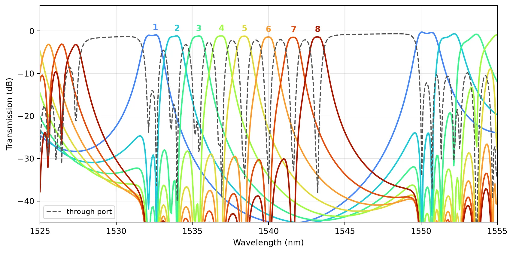

The numbers a link designer asks for are the channel spacing, the passband width, the drop loss, and how much of a neighbouring channel arrives at the wrong port.

for k in range(8):
    channel_db = 10 * np.log10(np.maximum(drops[k], 1e-12))
    # Peak of this channel, and what every other channel delivers at that same wavelength.
    i = np.where(in_band)[0][np.argmax(channel_db[in_band])]
    others = {j: 10 * np.log10(max(drops[j][i], 1e-12)) for j in range(8) if j != k}
    adjacent = [others[j] for j in (k - 1, k + 1) if j in others]
    distant = [v for j, v in others.items() if j not in (k - 1, k + 1)]
    # 3 dB passband, restricted to the neighbourhood of the peak.
    band = np.where((channel_db > channel_db[i] - 3) & (np.abs(lam_chip - lam_chip[i]) < 3.0))[0]
    print(f"OUT{k + 1}: peak {channel_db[i]:5.2f} dB at {lam_chip[i]:7.2f} nm, "
          f"3 dB width {lam_chip[band.max()] - lam_chip[band.min()]:.2f} nm, "
          f"adjacent crosstalk {max(adjacent):6.1f} dB, non-adjacent {max(distant):6.1f} dB")

OUT1: peak -0.91 dB at 1532.58 nm, 3 dB width 1.12 nm, adjacent crosstalk  -33.5 dB, non-adjacent  -46.9 dB
OUT2: peak -1.15 dB at 1534.00 nm, 3 dB width 0.98 nm, adjacent crosstalk  -20.8 dB, non-adjacent  -68.5 dB
OUT3: peak -1.18 dB at 1535.42 nm, 3 dB width 0.97 nm, adjacent crosstalk  -21.8 dB, non-adjacent  -32.2 dB
OUT4: peak -1.14 dB at 1536.92 nm, 3 dB width 0.82 nm, adjacent crosstalk  -22.5 dB, non-adjacent  -33.4 dB
OUT5: peak -1.22 dB at 1538.42 nm, 3 dB width 0.83 nm, adjacent crosstalk  -22.8 dB, non-adjacent  -33.8 dB
OUT6: peak -1.40 dB at 1540.00 nm, 3 dB width 0.82 nm, adjacent crosstalk  -23.2 dB, non-adjacent  -34.2 dB
OUT7: peak -1.47 dB at 1541.65 nm, 3 dB width 0.83 nm, adjacent crosstalk  -23.9 dB, non-adjacent  -34.5 dB
OUT8: peak -1.40 dB at 1543.22 nm, 3 dB width 0.82 nm, adjacent crosstalk  -22.9 dB, non-adjacent  -34.0 dB

Summary

The eight channels land between 1532.6 nm and 1543.2 nm on a 1.52 nm grid, on a routed block of $0.64 \times 1.76$ mm$^2$. The only geometry parameter that differs between stages is the phase-section length $L_t$, at about 0.04 nm of wavelength per nm of $L_t$. The drop loss, passband width, and crosstalk of each channel are printed above.

Moving the comb to a different grid means re-running the three-point calibration and the eight channel cavities. The circuit assembly and the routing are unchanged. The free spectral range of about 18 nm is the limit on how wide a comb one cavity design can carry.

Two numbers in the design are set by the etch rather than by the optics. The corrugation period follows from phase matching between the forward TE₀ and backward TE₁ modes, and the coupling gap of the mode demultiplexer has to clear the sidewall flare, which on a 200 nm ridge at 60 degrees removes 116 nm from each side of any gap drawn on the mask.

The same chip also works in reverse. Driving the OUT ports instead of IN multiplexes eight sources onto one waveguide, since every component in the path is reciprocal.