Avalanche Photodiode

Download notebook (.zip)

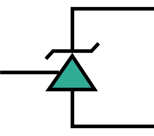
An avalanche photodiode (APD) is a photodiode with internal gain. Each photogenerated carrier is accelerated by a high reverse-bias field until it creates new electron-hole pairs by impact ionization, so the primary photocurrent $I_p = R_0 P$ is multiplied by a mean gain $M$. The AvalanchePhotodiodeTimeStepper models this device for time-domain simulations. The output current is

$$I = M\left(I_p + I_{d,\rm bulk}\right) + I_{d,\rm surf}$$

where $R_0$ is the primary responsivity at unity gain, $I_{d,\rm bulk}$ is the bulk dark current, which passes through the multiplication region and is multiplied with the signal, and $I_{d,\rm surf}$ is the surface dark current, which is not.

The gain is not free. Three effects set how much of it is useful:

• Bias dependence: $M$ rises steeply as the reverse bias approaches breakdown.
• Excess noise: impact ionization is a random process, so the shot noise grows faster than the signal, by the excess noise factor $F(M)$.
• Gain-bandwidth product: the avalanche takes time to build up, so above some gain the bandwidth falls as $1/M$.

This guide shows how to set up the model, how the gain follows the bias [1], how the bandwidth depends on the gain, how to find the gain that maximizes the signal-to-noise ratio [2], and how much an APD improves a 10 Gb/s receiver over a PIN photodiode. Basic detection with a PIN photodiode and a transimpedance amplifier (TIA) is covered in the Photodiode guide.

References

1. Miller, S. L. “Avalanche breakdown in germanium.” Physical Review 1955 99 (4), 1234-1241, doi: 10.1103/PhysRev.99.1234.
2. McIntyre, R. J. “Multiplication noise in uniform avalanche diodes.” IEEE Transactions on Electron Devices 1966 13 (1), 164-168, doi: 10.1109/T-ED.1966.15651.

Setup

import matplotlib.pyplot as plt
import numpy as np
import photonforge as pf
import photonforge.abstract as pfa
from math import erfc

viewer = pf.live_viewer.LiveViewer()

LiveViewer started at http://127.0.0.1:38909. Call its 'stop()' method to free the port.

The simulation constants come first. pf.C_0 is the speed of light in µm/s, so dividing it by a wavelength in µm gives the carrier frequency in Hz. The APD responds to optical power only, so the carrier frequency does not change its output, but every time-domain setup needs one. A time step of 1 ps resolves signals up to 500 GHz, far above the bandwidth of the device.

# Set the basic technology as the default for the abstract components
tech = pf.basic_technology()
pf.config.default_technology = tech

# Define the O-band carrier wavelength (µm) and its frequency (Hz)
lda0 = 1.31
f0 = pf.C_0 / lda0

z0 = 50.0  # Reference impedance of the electrical port (Ω)
q_e = 1.602176634e-19  # Elementary charge (C)
time_step = 1e-12  # Simulation time step (s)

The APD in this guide uses round, illustrative parameter values rather than those of a specific device:

• Primary responsivity: 0.6 A/W.
• Breakdown voltage: 30 V.
• Effective ionization ratio: $k = 0.1$.
• Gain-bandwidth product: 200 GHz.
• Intrinsic bandwidth: 10 GHz, the transit and RC limited bandwidth at low gain.
• Dark current: 0.1 µA of primary bulk dark current, which is multiplied, and 50 nA of surface dark current, which is not.

# Define the parameters of the APD
responsivity = 0.6  # Primary responsivity at unity gain (A/W)
breakdown_voltage = 30.0  # Breakdown voltage (V)
ionization_ratio = 0.1  # Effective ionization ratio k
gain_bandwidth_product = 200e9  # Gain-bandwidth product (Hz)
intrinsic_bandwidth = 10e9  # Transit and RC limited bandwidth (Hz)
bulk_dark_current = 0.1e-6  # Primary bulk dark current (A)
surface_dark_current = 50e-9  # Surface dark current (A)

Gain Against Bias

The multiplication of an APD is commonly described by Miller’s empirical formula [1]

$$M(V) = \left[1 - \left(\frac{V}{V_{\rm br}}\right)^n\right]^{-1}$$

where $V$ is the reverse bias, $V_{\rm br}$ the breakdown voltage and $n$ an exponent fitted to measurement. The function miller_gain tabulates this curve as an Interpolator, which is passed directly as the multiplication argument of the APD. Near breakdown the gain is clipped at max_multiplication (1000 by default), since the formula diverges there. For a device with separate absorption and multiplication layers, the optional punch_through_voltage holds the gain at 1 below the bias at which the absorber is depleted.

We use $n = 3$, within the range of 2 to 6 typical of measured junctions.

exponent = 3.0  # Miller exponent n

# Define a fine bias grid that stops just below breakdown (V)
biases = np.linspace(0, 29.95, 500)

# Tabulate the Miller gain curve on the bias grid
gain_curve = pf.miller_gain(
    biases, breakdown_voltage=breakdown_voltage, exponent=exponent
)

The avalanche_photodiode component from the abstract library uses the AvalanchePhotodiodeTimeStepper as its time-domain model. It has one optical input P0 and one electrical output E0, like the photodiode. With a gain curve as multiplication, the gain is read from the curve at bias. The bias is fixed during a simulation, so the gain is evaluated once when the time stepper is set up.

# Create the APD, with the gain read from the Miller curve at the given bias
apd = pfa.avalanche_photodiode(
    responsivity=responsivity,
    multiplication=gain_curve,
    bias=20.0,  # Reverse bias (V)
    bulk_dark_current=bulk_dark_current,
    dark_current=surface_dark_current,
    seed=0,  # Seed of the noise generator
)

# Display the component and its ports
viewer(apd)

A single component does not need a circuit around it: setup_time_stepper works on the APD directly, and the optical input is injected as a TimeSeries keyed by the port name P0@0. The input is the optical field amplitude $A$, with $\lvert A \rvert^2$ the power in W, so a constant power $P$ is the constant amplitude $\sqrt{P}$. The APD output current is recovered from the electrical wave amplitude as $I = \Re\{A\} \sqrt{Z_0} / G$, and with the default TIA gain $G$ of 1 V/A this is simply $\Re\{A\} \sqrt{Z_0}$.

We sweep the bias and record the mean output current twice at each point: once with 1 µW of light and once in the dark. The difference of the two, divided by the unity-gain photocurrent $R_0 P$, gives the gain. The first 1 ns of each run is discarded while the output filter settles.

power = 1e-6  # Optical input power (W)
num_steps = 20000  # Number of time steps per run
settled = slice(1000, None)  # Time steps kept after the output settles

# Define the bias points of the sweep (V)
sweep_biases = np.linspace(15, 29.8, 25)

# Create lists for the mean current with light and in the dark
light_current = []
dark_current = []

for bias in sweep_biases:
    # Update the bias and set up the time stepper at this bias
    apd.update(bias=bias)
    time_stepper = apd.setup_time_stepper(
        time_step=time_step, carrier_frequency=f0, show_progress=False
    )

    # Run once with light and once in the dark
    for p, currents in ((power, light_current), (0.0, dark_current)):
        # Reset the time stepper so that each run starts from the same state
        time_stepper.reset()

        # Build the input field amplitude for a constant optical power
        field = np.full(num_steps, np.sqrt(p), dtype=complex)
        inputs = pf.TimeSeries(values={"P0@0": field}, time_step=time_step)

        # Run the time-domain simulation
        output = time_stepper.step(
            inputs=inputs, time_step=time_step, show_progress=False
        )

        # Convert the output wave amplitude to current, for a TIA gain of 1 V/A
        current = np.real(output["E0@0"]) * np.sqrt(z0)

        # Store the mean current after the output settles
        currents.append(current[settled].mean())

# Convert the current lists to arrays
light_current = np.array(light_current)
dark_current = np.array(dark_current)

# Extract the gain from the photocurrent above the dark current
measured_gain = (light_current - dark_current) / (responsivity * power)

# Plot the currents with light and in the dark against bias
fig, (ax1, ax2) = plt.subplots(1, 2, figsize=(9, 3.5), tight_layout=True)
ax1.semilogy(sweep_biases, light_current * 1e6, "o-", ms=4, label="Light, 1 µW")
ax1.semilogy(sweep_biases, dark_current * 1e6, "o-", ms=4, label="Dark")
ax1.set(xlabel="Reverse bias (V)", ylabel="Current (µA)")
ax1.legend()

# Plot the extracted gain with the Miller curve for comparison
ax2.semilogy(sweep_biases, measured_gain, "o", ms=4, label="From simulation")
ax2.semilogy(biases, gain_curve(biases), "k-", alpha=0.5, label="Miller curve")
ax2.set(xlabel="Reverse bias (V)", ylabel="Gain M", xlim=(15, 30), ylim=(0.8, 200))
_ = ax2.legend()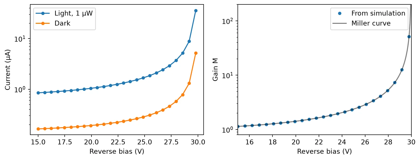

Both currents rise with the gain as the bias approaches breakdown, the dark current more slowly because its surface part is not multiplied. The gain extracted from the two currents follows the Miller curve that was passed to the model.

Bandwidth and Gain-Bandwidth Product

At low gain the APD bandwidth is set by the carrier transit time and the RC time constant, as in a PIN photodiode. At high gain the avalanche needs several transits to build up, and the bandwidth falls as ${\rm GBP}/M$, where GBP is the gain-bandwidth product. The model combines the two limits into a single first-order response with the 3 dB bandwidth

$$\frac{1}{f_{\rm 3dB}^2} = \frac{1}{f_{\rm int}^2} + \left(\frac{M}{\rm GBP}\right)^2$$

with $f_{\rm int}$ set by intrinsic_bandwidth and GBP by gain_bandwidth_product. The crossover between the two regimes is at $M = {\rm GBP}/f_{\rm int} = 20$ for this device.

To measure the frequency response, the input power is modulated with several tones at once:

$$P(t) = P_0 \left[1 + \frac{m}{N}\sum_{j=1}^{N} \cos\left(2\pi f_j t\right)\right]$$

The photocurrent is linear in optical power, so each tone is detected independently of the others. Its amplitude in the output current, divided by the amplitude $M R_0 P_0 m / N$ it would have without a bandwidth limit, gives the normalized response $\lvert H(f_j) \rvert$. Each tone frequency is placed on an exact bin of the discrete Fourier transform of the record, so each tone is read from a single bin without spectral leakage. We use eight tones between 1 and 60 GHz, an average power of 10 µW and a total modulation depth $m = 0.8$, which keeps the power positive at all times.

# Create an APD with both bandwidth limits and no dark current
apd_bw = pfa.avalanche_photodiode(
    responsivity=responsivity,
    ionization_ratio=ionization_ratio,
    gain_bandwidth_product=gain_bandwidth_product,
    intrinsic_bandwidth=intrinsic_bandwidth,
    seed=0,
)

num_steps = 2**19  # Number of time steps in the record
average_power = 10e-6  # Average optical input power (W)
modulation_index = 0.8  # Total modulation depth, shared equally by the tones

# Place the tone frequencies on exact Fourier bins of the record
record = num_steps * time_step
tone_bins = np.round(np.geomspace(1e9, 60e9, 8) * record).astype(int)
tones = tone_bins / record
tone_depth = modulation_index / tones.size

# Build the multi-tone input power and convert it to field amplitude
t = np.arange(num_steps) * time_step
modulation = np.cos(2 * np.pi * tones[:, None] * t).sum(axis=0)
power_t = average_power * (1 + tone_depth * modulation)
inputs = pf.TimeSeries(values={"P0@0": np.sqrt(power_t) + 0j}, time_step=time_step)

# Define the gains to compare and a fine frequency grid for the analytic response
gains = [5, 20, 40, 80]
freq_fine = np.geomspace(0.5e9, 80e9, 300)

fig, (ax1, ax2) = plt.subplots(1, 2, figsize=(9, 3.5), tight_layout=True)
for i, gain in enumerate(gains):
    # Update the gain and run the time-domain simulation
    apd_bw.update(multiplication=float(gain))
    time_stepper = apd_bw.setup_time_stepper(
        time_step=time_step, carrier_frequency=f0, show_progress=False
    )
    output = time_stepper.step(inputs=inputs, time_step=time_step, show_progress=False)

    # Convert the output wave amplitude to current, for a TIA gain of 1 V/A
    current = np.real(output["E0@0"]) * np.sqrt(z0)

    # Read each tone amplitude from its Fourier bin and normalize it
    tone_amplitude = 2 * np.abs(np.fft.rfft(current)[tone_bins]) / num_steps
    response = tone_amplitude / (gain * responsivity * average_power * tone_depth)

    # Compute the combined 3 dB bandwidth and the analytic first-order response
    f_3db = 1 / np.sqrt(
        1 / intrinsic_bandwidth**2 + (gain / gain_bandwidth_product) ** 2
    )
    response_theory = 1 / np.sqrt(1 + (freq_fine / f_3db) ** 2)
    print(f"M = {gain}: 3 dB bandwidth {f_3db / 1e9:.1f} GHz")

    # Plot the simulated tones with the analytic response for comparison
    label = f"M = {gain}"
    ax1.semilogx(tones / 1e9, 20 * np.log10(response), "o", color=f"C{i}", label=label)
    ax1.semilogx(
        freq_fine / 1e9, 20 * np.log10(response_theory), "-", color=f"C{i}", alpha=0.5
    )

    # Mark this gain on the bandwidth curve
    ax2.loglog(gain, f_3db / 1e9, "o", color=f"C{i}")

# Mark the 3 dB level on the response plot
ax1.axhline(-3, color="k", ls=":", lw=1)
ax1.set(xlabel="Modulation frequency (GHz)", ylabel="Normalized response (dB)")
ax1.legend(fontsize=8)

# Compute the combined bandwidth over a wide range of gain
gain_fine = np.geomspace(1, 200, 200)
f_3db_fine = 1 / np.sqrt(
    1 / intrinsic_bandwidth**2 + (gain_fine / gain_bandwidth_product) ** 2
)

# Plot the combined bandwidth with its intrinsic and GBP / M limits
ax2.loglog(gain_fine, f_3db_fine / 1e9, "k-", alpha=0.6, label="Combined")
ax2.loglog(
    gain_fine,
    np.full_like(gain_fine, intrinsic_bandwidth / 1e9),
    "k:",
    label="Intrinsic",
)
ax2.loglog(gain_fine, gain_bandwidth_product / gain_fine / 1e9, "k--", label="GBP / M")
ax2.set(xlabel="Gain M", ylabel="3 dB bandwidth (GHz)", ylim=(1, 30))
_ = ax2.legend(fontsize=8)

M = 5: 3 dB bandwidth 9.7 GHz
M = 20: 3 dB bandwidth 7.1 GHz
M = 40: 3 dB bandwidth 4.5 GHz
M = 80: 3 dB bandwidth 2.4 GHz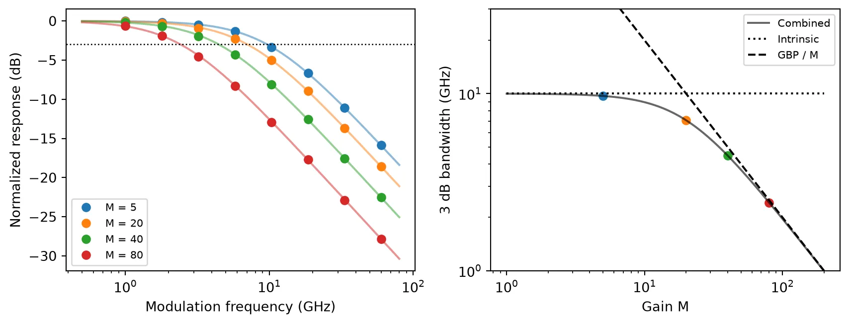

On the left, the simulated tone amplitudes follow the first-order response for each gain, plotted as lines for reference. On the right, the bandwidth stays near $f_{\rm int} = 10$ GHz (dotted line) up to a gain of about 10 and then approaches the ${\rm GBP}/M$ asymptote (dashed line). Setting either argument to zero removes that limit, and setting both to zero gives an APD with no bandwidth limit.

Excess Noise and the Optimum Gain

Impact ionization is a random process: each primary carrier is multiplied by a random number whose mean is $M$. The shot noise therefore grows as $M^2 F(M)$ instead of $M^2$. McIntyre’s excess noise factor [2] is

$$F(M) = k M + \left(1 - k\right)\left(2 - \frac{1}{M}\right)$$

where $k$ is the ratio of the hole to electron ionization coefficients, set by ionization_ratio. For $k = 0$ only one carrier type ionizes and $F$ saturates at 2. For $k = 1$ both ionize equally and $F$ grows as $M$. The one-sided current noise power spectral density (PSD) at the APD output is

$$S_I = 2q\left[M^2 F(M)\left(I_p + I_{d,\rm bulk}\right) + I_{d,\rm surf}\right] + S_{\rm th}$$

where $q$ is the elementary charge and $S_{\rm th}$ is the input-referred thermal noise PSD of the TIA, set by thermal_noise.

The signal current is $M I_p$, so for a CW input the signal-to-noise ratio (SNR) is

$$\mathrm{SNR}(M) = \frac{M^2 I_p^2}{S_I\,B_n}$$

where $B_n$ is the noise bandwidth. For a first-order response $B_n = \pi f_{\rm 3dB} / 2$. Without dark current, setting $d\,\mathrm{SNR}/dM = 0$ gives the gain that maximizes the SNR as the root of

$$k M^3 + \left(1 - k\right) M = \frac{S_{\rm th}}{q I_p}$$

At low gain the multiplied signal rises above the fixed thermal noise and the SNR improves as $M^2$. At high gain the multiplied shot noise dominates, and since it grows faster than the signal, the SNR falls again. The optimum gain is higher for a small $k$ and for a large thermal noise.

We compare three values of $k$: 0.02, typical of silicon, 0.1 for the APD of this guide, and 0.5, typical of InP. The input power is -29 dBm and the thermal noise is 15 pA/√Hz, a typical input-referred noise for a 10 Gb/s TIA. To keep the same noise bandwidth at every gain, the gain-bandwidth limit is left out here and only intrinsic_bandwidth is set. The SNR is measured directly from the output current as its squared mean divided by its variance.

power = 10 ** (-29 / 10) * 1e-3  # Optical input power (W)
thermal_asd = 15e-12  # Input-referred thermal noise of the TIA (A/√Hz)
num_steps = 2**17  # Number of time steps per run
settled = slice(1000, None)  # Time steps kept after the output settles

# Compute the primary photocurrent, the thermal noise PSD and the noise bandwidth
primary_current = responsivity * power
thermal_noise = thermal_asd**2
noise_bandwidth = np.pi / 2 * intrinsic_bandwidth

# Build the input field amplitude for a constant optical power
field = np.full(num_steps, np.sqrt(power), dtype=complex)
inputs = pf.TimeSeries(values={"P0@0": field}, time_step=time_step)

# Define the ionization ratios to compare
materials = {"Silicon": 0.02, "This APD": ionization_ratio, "InP": 0.5}

# Define the simulated gains and a fine gain grid for the analytic SNR
gains = np.geomspace(1, 100, 13)
gain_fine = np.geomspace(1, 100, 300)

# Create a dictionary for the optimum gain of each material
optimum_gain = {}

fig, ax = plt.subplots(figsize=(7, 3.5), tight_layout=True)
for i, (name, k) in enumerate(materials.items()):
    # Create an APD with this ionization ratio and only the intrinsic bandwidth
    apd_noise = pfa.avalanche_photodiode(
        responsivity=responsivity,
        ionization_ratio=k,
        intrinsic_bandwidth=intrinsic_bandwidth,
        thermal_noise=thermal_noise,
        seed=0,
    )

    snr = []
    for gain in gains:
        # Update the gain and run the time-domain simulation
        apd_noise.update(multiplication=float(gain))
        time_stepper = apd_noise.setup_time_stepper(
            time_step=time_step, carrier_frequency=f0, show_progress=False
        )
        output = time_stepper.step(
            inputs=inputs, time_step=time_step, show_progress=False
        )

        # Convert the output to current and compute its SNR
        current = np.real(output["E0@0"])[settled] * np.sqrt(z0)
        snr.append(current.mean() ** 2 / current.var())

    # Compute the analytic SNR from the excess noise factor
    excess = k * gain_fine + (1 - k) * (2 - 1 / gain_fine)
    shot = 2 * q_e * gain_fine**2 * excess * primary_current
    snr_theory = (gain_fine * primary_current) ** 2 / (
        (shot + thermal_noise) * noise_bandwidth
    )

    # Solve the cubic for the optimum gain and keep its real positive root
    roots = np.roots([k, 0, 1 - k, -thermal_noise / (q_e * primary_current)])
    m_opt = roots[np.isreal(roots) & (roots.real > 0)].real[0]
    optimum_gain[name] = m_opt

    # Plot the simulated and analytic SNR, and mark the optimum gain
    label = f"{name}, k = {k}"
    ax.semilogx(gains, 10 * np.log10(snr), "o", color=f"C{i}", label=label)
    ax.semilogx(gain_fine, 10 * np.log10(snr_theory), "-", color=f"C{i}", alpha=0.5)
    ax.axvline(m_opt, color=f"C{i}", ls=":", lw=1)

    # Compare the best SNR with the SNR at unity gain
    improvement = 10 * np.log10(snr_theory.max() / snr_theory[0])
    print(f"{label}: optimum gain {m_opt:.1f}, SNR improvement {improvement:.1f} dB")

ax.set(xlabel="Gain M", ylabel="SNR (dB)")
_ = ax.legend(fontsize=8)

Silicon, k = 0.02: optimum gain 44.9, SNR improvement 24.5 dB
This APD, k = 0.1: optimum gain 26.4, SNR improvement 22.1 dB
InP, k = 0.5: optimum gain 15.5, SNR improvement 18.7 dB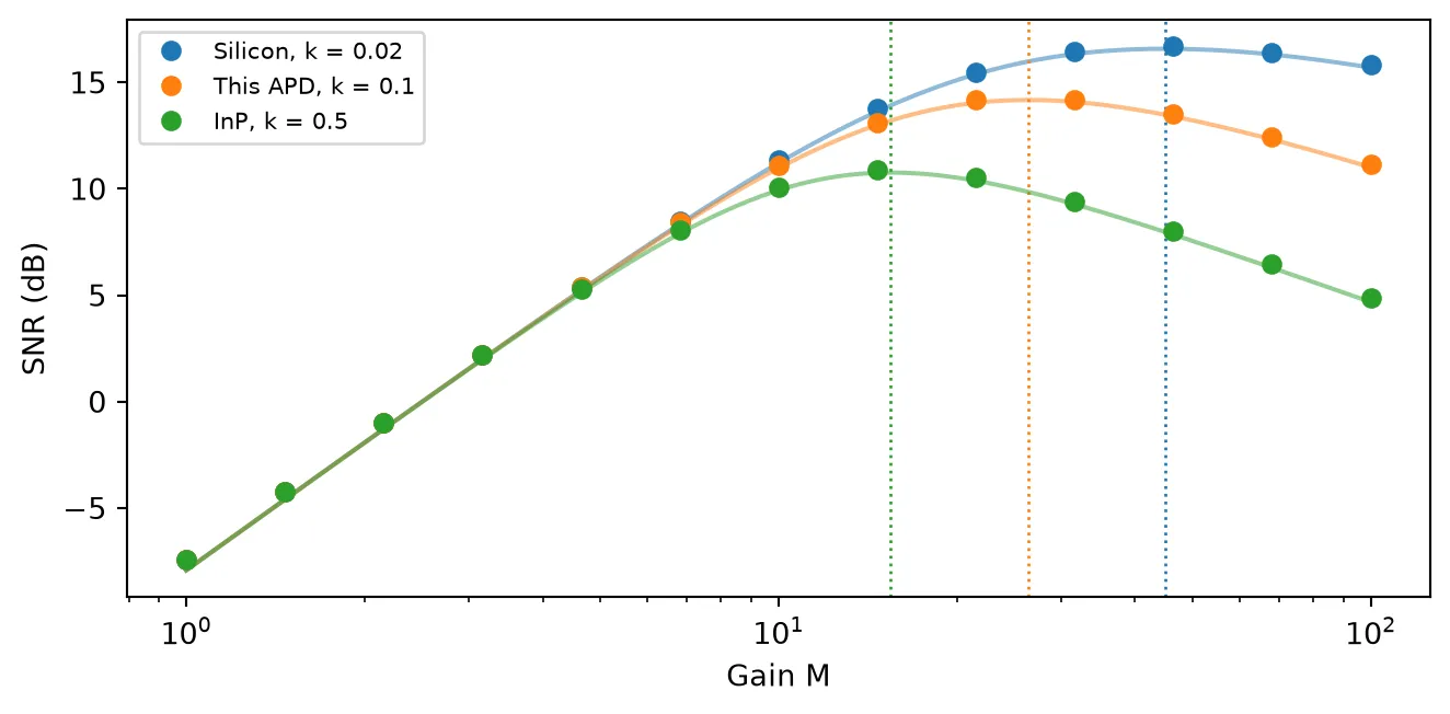

The markers are the SNR of the simulated output current and the lines the analytic SNR, with the optimum gain of each material marked by a dotted line. All three curves start from the same thermally limited SNR at $M = 1$, where the APD behaves as a PIN photodiode, since $F(1) = 1$. The lower the ionization ratio, the further the gain can be raised before the excess noise takes over, and the larger the improvement. The optimum also depends on the TIA noise, and rises with it.

Two other noise contributions follow the same equation. bulk_dark_current is multiplied and carries the same $M^2 F(M)$ penalty as the signal, while dark_current, the surface part, adds unmultiplied shot noise.

Receiver Sensitivity at 10 Gb/s

Finally, we compare two receivers detecting a 10 Gb/s non-return-to-zero (NRZ) signal at an average power of -29 dBm:

• A PIN photodiode, modeled with the photodiode component, with the same responsivity, bandwidth, dark current and TIA noise as the APD at unity gain.
• The APD, with its full set of parameters, biased at the voltage that gives the optimum gain found above. The bias is found by inverting the Miller curve.

The transmitter is ideal: the power is $2 P_{\rm avg}$ for a one and zero for a zero, with instantaneous transitions, so any closure of the eye comes from the receiver. The eye opening is quantified by the Q factor,

$$Q = \frac{\mu_1 - \mu_0}{\sigma_1 + \sigma_0}$$

where $\mu$ and $\sigma$ are the mean and standard deviation of the current sampled in the ones and in the zeros. For Gaussian noise the bit error ratio is $\mathrm{BER} = \frac{1}{2}\,\mathrm{erfc}\left(Q/\sqrt{2}\right)$. The best sampling instant is found by evaluating Q at every time step within one bit and keeping the largest. In the eye diagrams it is marked by a dashed line.

# Find the bias of the optimum gain by inverting the Miller curve
m_opt = optimum_gain["This APD"]
bias_opt = np.interp(m_opt, gain_curve(biases), biases)
print(f"Optimum gain {m_opt:.1f} at a bias of {bias_opt:.2f} V")

# Create the PIN and APD receivers with the same responsivity and TIA noise
receivers = {
    "PIN photodiode": pfa.photodiode(
        responsivity=responsivity,
        filter_frequency=intrinsic_bandwidth,
        dark_current=bulk_dark_current + surface_dark_current,
        thermal_noise=thermal_noise,
        seed=0,
    ),
    "Avalanche photodiode": pfa.avalanche_photodiode(
        responsivity=responsivity,
        multiplication=gain_curve,
        bias=bias_opt,
        ionization_ratio=ionization_ratio,
        gain_bandwidth_product=gain_bandwidth_product,
        intrinsic_bandwidth=intrinsic_bandwidth,
        bulk_dark_current=bulk_dark_current,
        dark_current=surface_dark_current,
        thermal_noise=thermal_noise,
        seed=0,
    ),
}

bit_rate = 10e9  # Bit rate (b/s)
num_bits = 1024  # Number of bits in the sequence
skip_bits = 8  # Number of bits discarded while the receiver settles
num_eye_bits = 300  # Number of bits overlaid in each eye diagram

# Build a random NRZ bit sequence as optical power and convert it to field amplitude
samples_per_bit = int(round(1 / bit_rate / time_step))
rng = np.random.default_rng(1)
bits = rng.integers(0, 2, num_bits)
power_t = np.repeat(2 * power * bits, samples_per_bit)
inputs = pf.TimeSeries(values={"P0@0": np.sqrt(power_t) + 0j}, time_step=time_step)

# Define the time axis of a two-bit window that starts half a bit early
half_bit = samples_per_bit // 2
eye_time = (np.arange(2 * samples_per_bit) - half_bit) * time_step

fig, axes = plt.subplots(1, 2, figsize=(9, 3.5), tight_layout=True)
for ax, (name, receiver) in zip(axes, receivers.items()):
    # Run the time-domain simulation for this receiver
    time_stepper = receiver.setup_time_stepper(
        time_step=time_step, carrier_frequency=f0, show_progress=False
    )
    output = time_stepper.step(inputs=inputs, time_step=time_step, show_progress=False)

    # Convert the output wave amplitude to current, for a TIA gain of 1 V/A
    current = np.real(output["E0@0"]) * np.sqrt(z0)

    # Arrange the current in one row per bit and split the rows into ones and zeros
    samples = current.reshape(num_bits, samples_per_bit)[skip_bits:]
    ones = samples[bits[skip_bits:] == 1]
    zeros = samples[bits[skip_bits:] == 0]

    # Evaluate Q at every sampling instant within the bit and keep the best
    q_factor = (ones.mean(0) - zeros.mean(0)) / (ones.std(0) + zeros.std(0))
    phase = int(np.argmax(q_factor))
    q_best = q_factor[phase]

    # Estimate the bit error ratio from Q for Gaussian noise
    ber = 0.5 * erfc(q_best / np.sqrt(2))
    print(f"{name}: Q = {q_best:.2f}, BER = {ber:.1e}")

    # Overlay the two-bit windows to draw the eye diagram
    for b in range(skip_bits, num_eye_bits):
        start = b * samples_per_bit - half_bit
        window = current[start : start + 2 * samples_per_bit]
        ax.plot(eye_time * 1e12, window * 1e6, color="C0", alpha=0.05)

    # Mark the best sampling instant
    ax.axvline(phase * time_step * 1e12, color="k", ls="--", lw=1)
    ax.set(xlabel="Time (ps)", ylabel="Current (µA)", title=f"{name}, Q = {q_best:.1f}")

Optimum gain 26.4 at a bias of 29.61 V
PIN photodiode: Q = 0.43, BER = 3.3e-01
Avalanche photodiode: Q = 6.83, BER = 4.3e-12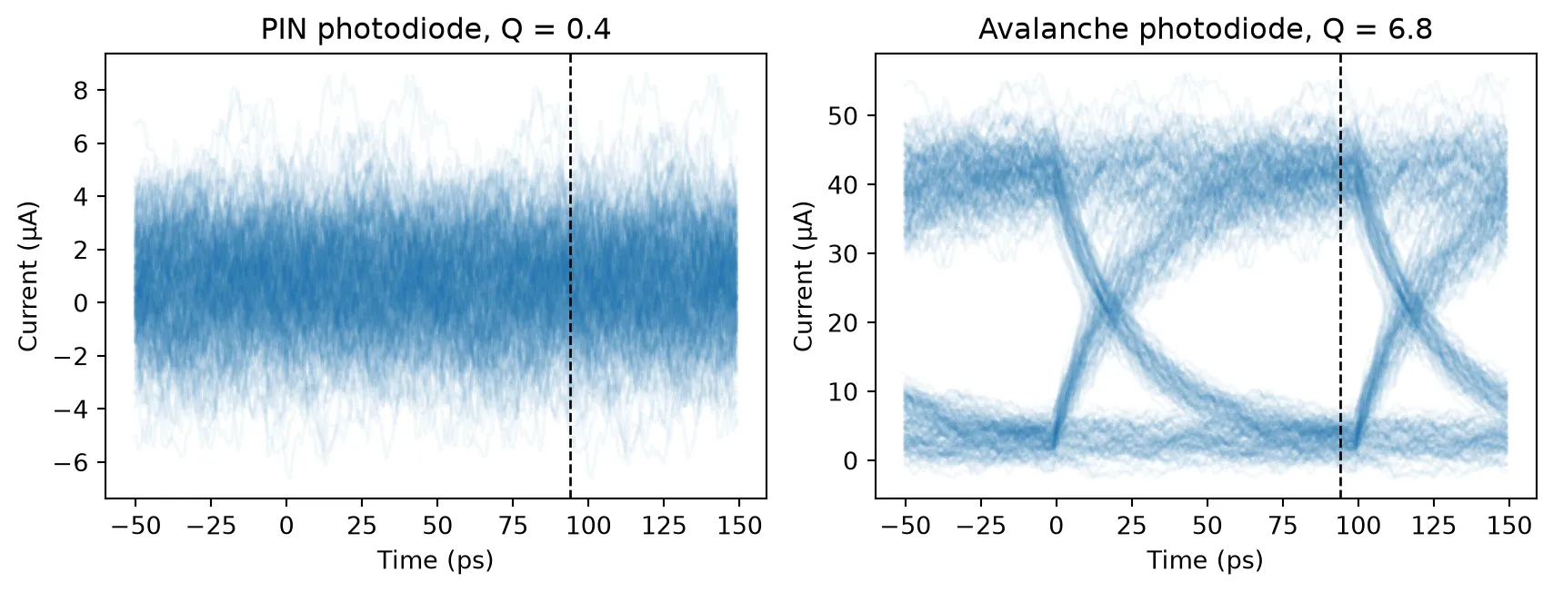

At -29 dBm the PIN receiver is limited by the thermal noise of the TIA. The photocurrent of a one is about 1.5 µA, below the thermal noise current of about 1.9 µA rms in the receiver bandwidth, and the eye is closed. The APD multiplies the photocurrent by its optimum gain before the TIA adds its noise, which opens the eye to a Q factor above 6, a BER below 10⁻¹⁰. The bandwidth reduction that comes with the gain, from 10 GHz to about 6 GHz, still leaves the eye open at 10 Gb/s.

With a first-order response, the current of a one keeps rising until the next transition, so the best sampling instant falls late in the bit rather than at the center of the eye.

The same receiver can be placed at the end of any link built from abstract components, such as a modulated laser, a fiber and an optical amplifier, in the same way as the PIN photodiode.

Summary

• pfa.avalanche_photodiode models an APD whose output current is $M(I_p + I_{d,\rm bulk}) + I_{d,\rm surf}$, exposed at the electrical port through the TIA gain as the wave amplitude $G I / \sqrt{Z_0}$.
• multiplication sets the gain as a number, or as an interpolator of gain against bias evaluated at bias. miller_gain tabulates Miller’s formula [1], with punch_through_voltage and max_multiplication bounding the curve.
• intrinsic_bandwidth and gain_bandwidth_product set a first-order response whose 3 dB bandwidth is flat at low gain and falls as ${\rm GBP}/M$ at high gain.
• ionization_ratio sets McIntyre’s excess noise factor $F(M)$ [2]. Together with thermal_noise it determines the gain that maximizes the SNR, which is higher for a smaller ionization ratio.
• bulk_dark_current is multiplied with the signal and dark_current is not. saturation_current and roll_off model space-charge saturation of the multiplied current, as in the Photodiode guide, and seed makes noise realizations reproducible.