Spiral Waveguide
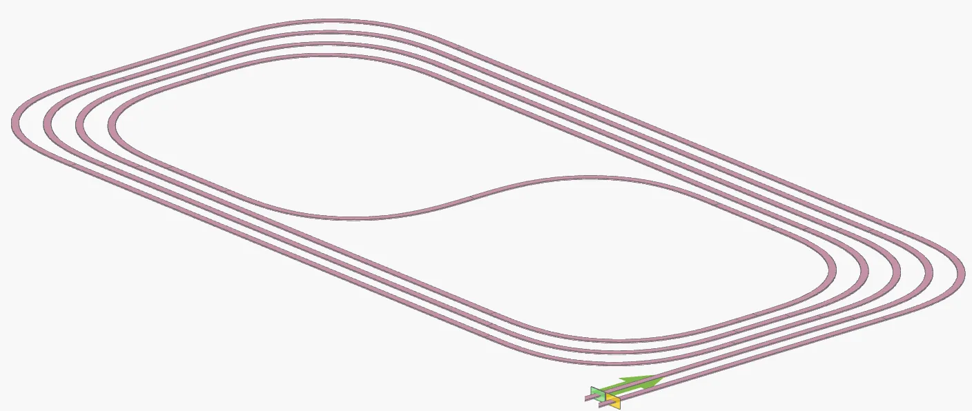
Simulating large photonic structures such as spirals using full-field electromagnetic methods like FDTD can be computationally expensive and time-consuming. This notebook demonstrates how we can efficiently simulate such devices using a compact circuit model, which leverages pre-characterized components—such as bends and straights—to drastically reduce simulation cost without compromising accuracy.
We begin by defining a custom silicon nitride (SiN) technology that includes both optical and electrical material properties, as well as port and layer specifications. We then construct a rectangular spiral waveguide with a total length of 5 mm and use a circuit-level simulation approach to compute its scattering matrix. The circuit model automatically performs one-time simulations for each unique waveguide element (e.g., a representative bend or straight) and assembles the global response based on their interconnections.
To validate the accuracy of the circuit model, we also define a full Tidy3D FDTD model for the spiral. While running this simulation is expensive, we provide a precomputed S-matrix file that users can download and use directly. This allows for a side-by-side comparison of the circuit and full-field results, highlighting the efficiency and effectiveness of the circuit-based approach for large passive photonic structures.
import matplotlib.pyplot as pltimport numpy as npimport photonforge as pfimport tidy3d as tdfrom photonforge.live_viewer import LiveViewer
viewer = LiveViewer()
LiveViewer started at http://127.0.0.1:33423. Call its 'stop()' method to free the port.Custom Silicon Nitride Technology
Section titled “Custom Silicon Nitride Technology”We begin by defining a custom silicon nitride (SiN) technology.
_Medium = td.components.medium.MediumType
def sin_technology(    sin_thickness=0.4,    sio2: dict[str, _Medium] = {        "optical": td.material_library["SiO2"]["Palik_Lossless"],        "electrical": td.Medium(permittivity=4.2, name="SiO2"),    },    sin: dict[str, _Medium] = {        "optical": td.material_library["Si3N4"]["Luke2015PMLStable"],        "electrical": td.Medium(permittivity=7.5, name="Si3N4"),    },):    """    Creates a custom silicon nitride (SiN) technology for photonic circuit simulation.
    Parameters:        sin_thickness (float): Thickness of the SiN core in microns.        sio2 (dict[str, Medium]): Dictionary with 'optical' and 'electrical' properties for the SiO2 cladding.        sin (dict[str, Medium]): Dictionary with 'optical' and 'electrical' properties for the SiN core.
    Returns:        pf.Technology: A fully defined technology object for layout and simulation.    """    # Define the layer for the SiN waveguide    layers = {        "WG": pf.LayerSpec((0, 0), description="SiN", color="#6db5dd18", pattern="/")    }
    # Define a mask at the base level for the SiN layer    sin_mask = pf.MaskSpec((0, 0))
    # Extrude the mask vertically to form the waveguide core    extrusion_specs = [        pf.ExtrusionSpec(            sin_mask, limits=(0, sin_thickness), medium=sin, sidewall_angle=0        )    ]
    # Define ports for a 3500 nm wide strip waveguide    ports = {        "Strip_3500": pf.PortSpec(            description="Strip waveguide, TE, 3500 nm wide",            width=10,            limits=(-2.5, sin_thickness + 2.5),            num_modes=1,            target_neff=2,            path_profiles=[(3.5, 0, (0, 0))],        ),    }
    # Assemble and return the full technology definition    tech = pf.Technology(        name="Custom SiN",        version="1.0",        layers=layers,        extrusion_specs=extrusion_specs,        ports=ports,        background_medium=sio2,    )    return tech
14:28:59 -03 WARNING: The material-library variant 'Palik_Lossless' is deprecated and maps to 'Palik_LowLoss' because it contains a tiny fitted loss despite its name. Use 'Palik_NoLoss' where available for a zero-loss Palik model.
Next, we initialize the custom SiN technology and set it as the default technology. To reduce simulation cost, especially for large structures like spirals, we also set a relatively coarse mesh refinement value.
# Instantiate the custom SiN technologytech = sin_technology()
# Set it as the default technology for PhotonForgepf.config.default_technology = tech
# Define default mesh refinementpf.config.default_mesh_refinement = 14
# Define a range of wavelengthswavelengths = np.linspace(1.5, 1.6, 51)freqs = pf.C_0 / wavelengths
Inspecting Port Modes
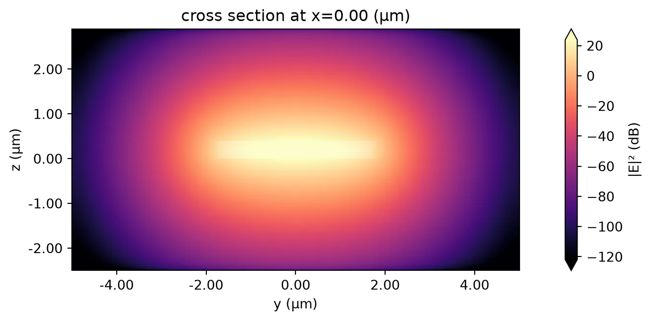
Section titled “Inspecting Port Modes”To improve the accuracy of the circuit model, we include the second-order mode by setting num_modes = 2. This is particularly important for large or tightly bent structures where higher-order modes may contribute significantly. We then visualize the mode to verify that the field is well confined and the mode shape and effective index are physically reasonable.
# Access the port specification for the 3500 nm wide stripport_spec = tech.ports["Strip_3500"]
# Interaction with second mode should be included in circuit analysisport_spec.num_modes = 2
# Solve for the port modes at a representative frequency (λ = 1.55 µm)mode_solver = pf.port_modes(    port_spec,    frequencies=[pf.C_0 / 1.55],    mesh_refinement=40,)
# Plot the electric field magnitude (in dB) (change the mode_index to inspect different modes)_, ax = plt.subplots(1, 1, figsize=(10, 3.5), tight_layout=True)_ = mode_solver.plot_field("E", "abs^2", "dB", mode_index=0, f=pf.C_0 / 1.55, ax=ax)
# Output mode data as a DataFramemode_solver.data.to_dataframe()
Uploading task 'Mode-ModeSolver…'Starting task 'Mode-ModeSolver': https://tidy3d.simulation.cloud/workbench?taskId=mo-241f2773-33c0-4afc-872b-1bbccb98289aDownloading data from 'Mode-ModeSolver'…| wavelength | n eff | k eff | loss (dB/cm) | TE (Ey) fraction | wg TE fraction | wg TM fraction | mode area | ||
|---|---|---|---|---|---|---|---|---|---|
| f | mode_index | ||||||||
| 1.934145e+14 | 0 | 1.55 | 1.733006 | 0.0 | 0.0 | 0.999870 | 0.987044 | 0.880759 | 1.706345 |
| 1 | 1.55 | 1.696169 | 0.0 | 0.0 | 0.999392 | 0.949150 | 0.885144 | 1.848523 |
Spiral Simulation
Section titled “Spiral Simulation”Creating a Spiral
Section titled “Creating a Spiral”We now create a rectangular spiral waveguide with a total length of 5000 µm using the parametric.rectangular_spiral function. The spiral is built from straight and bent waveguide segments, with 80 µm bend radius and 10.5 µm separation between waveguide centers. We also specify Tidy3D as the active bend model with an Euler bend profile. Finally, we visualize the spiral layout to verify its structure.
pf.parametric.rectangular_spiral??# Define total spiral length in micronsspiral_length = 5000
# Create the rectangular spiral geometry using the specified port and bend settingsspiral = pf.parametric.rectangular_spiral( port_spec=port_spec, radius=80, full_length=spiral_length, separation=10.5, align_ports="x", bend_kwargs={ "model": pf.Tidy3DModel(port_symmetries=[("P1", "P0")]), "euler_fraction": 0.5, },)
# Visualize the spiral layoutviewer(spiral);fill:%23221f20;font-weight:bold;font-size:21.140988px;}.terminal{fill:none;stroke:%23805080;stroke-width:2.642624;}.dashed{stroke-dasharray:13.213118,7.927871;}.port{fill:none;stroke:%23805080;stroke-width:5.285247;}.virtual-connection{fill:none;stroke:%23907090;stroke-width:3.963935;}.layer_0_0{stroke:%235b98b9;fill:url(%23pat-layer_0_0);fill-opacity:0.492;}.label_0_0{fill:%235b98b9;}</style><defs><path id=%22port-symbol%22 class=%22port%22 d=%22M 0,-10.570494 L 15.855741,0 0,10.570494%22 /><path id=%22ref-port-symbol%22 class=%22port%22 style=%22stroke-opacity:0.33;%22 d=%22M 0,-7.927871 C 10.570494,-7.927871 10.570494,7.927871 0,7.927871%22 /><circle id=%22port-bend-symbol%22 style=%22stroke-width:0;stroke:none;fill:%23805080;fill-opacity:1;%22 cx=%220%22 cy=%220%22 r=%224.756722%22 /><circle id=%22connection-symbol%22 style=%22stroke-width:0;stroke:none;fill:%23907090;fill-opacity:1;%22 cx=%220%22 cy=%220%22 r=%225.549509%22 /><pattern id=%22pat-layer_0_0%22 patternUnits=%22userSpaceOnUse%22 width=%2213.213118%22 height=%2213.213118%22 patternTransform=%22translate(0.000000,0.000000)%22><line x1=%220%22 y1=%220%22 x2=%2213.213118%22 y2=%2213.213118%22 style=%22stroke:%235b98b9;stroke-width:1.321312%22 /><line x1=%22-6.606559%22 y1=%226.606559%22 x2=%226.606559%22 y2=%2219.819676%22 style=%22stroke:%235b98b9;stroke-width:1.321312%22 /><line x1=%226.606559%22 y1=%22-6.606559%22 x2=%2219.819676%22 y2=%226.606559%22 style=%22stroke:%235b98b9;stroke-width:1.321312%22 /></pattern><g id=%22C1%22 data-name=%22bend__AGMWRVKHS2IZZPX4KFTRZNJQARHWRMUOC2B7ESZGZKZYPVNYCLAQ%22><path class=%22layer_0_0%22 d=%22M 0.000000,-1.750000 4.153000,-1.755000 6.225000,-1.766000 8.294000,-1.788000 10.360000,-1.824000 12.422000,-1.878000 14.481000,-1.954000 16.535000,-2.054000 18.585000,-2.182000 20.630000,-2.341000 22.668000,-2.536000 23.685000,-2.647000 24.700000,-2.769000 25.713000,-2.901000 26.723000,-3.044000 27.731000,-3.197000 28.737000,-3.363000 29.739000,-3.540000 30.739000,-3.730000 31.735000,-3.933000 32.728000,-4.149000 33.717000,-4.378000 34.702000,-4.621000 35.683000,-4.879000 36.659000,-5.151000 37.629000,-5.438000 38.595000,-5.740000 39.554000,-6.058000 40.507000,-6.391000 41.454000,-6.741000 42.394000,-7.107000 43.326000,-7.490000 44.251000,-7.890000 45.168000,-8.307000 46.078000,-8.740000 46.979000,-9.190000 47.872000,-9.657000 48.756000,-10.140000 49.631000,-10.640000 50.497000,-11.155000 51.353000,-11.686000 52.199000,-12.233000 53.036000,-12.795000 53.861000,-13.373000 54.676000,-13.966000 55.480000,-14.573000 56.272000,-15.196000 57.053000,-15.833000 57.822000,-16.484000 58.579000,-17.149000 59.323000,-17.828000 60.055000,-18.520000 60.774000,-19.226000 61.480000,-19.945000 62.172000,-20.677000 62.851000,-21.421000 63.516000,-22.178000 64.167000,-22.947000 64.804000,-23.728000 65.427000,-24.520000 66.034000,-25.324000 66.627000,-26.139000 67.205000,-26.964000 67.767000,-27.801000 68.314000,-28.647000 68.845000,-29.503000 69.360000,-30.369000 69.860000,-31.244000 70.343000,-32.128000 70.810000,-33.021000 71.260000,-33.922000 71.693000,-34.832000 72.110000,-35.749000 72.510000,-36.674000 72.893000,-37.606000 73.259000,-38.546000 73.609000,-39.493000 73.942000,-40.446000 74.260000,-41.405000 74.562000,-42.371000 74.849000,-43.341000 75.121000,-44.317000 75.379000,-45.298000 75.622000,-46.283000 75.851000,-47.272000 76.067000,-48.265000 76.270000,-49.261000 76.460000,-50.261000 76.637000,-51.263000 76.803000,-52.269000 76.956000,-53.277000 77.099000,-54.287000 77.231000,-55.300000 77.353000,-56.315000 77.566000,-58.350000 77.743000,-60.392000 77.886000,-62.439000 78.000000,-64.492000 78.087000,-66.548000 78.151000,-68.609000 78.196000,-70.673000 78.224000,-72.740000 78.241000,-74.810000 78.250000,-78.961000 78.250000,-80.000000 81.750000,-80.000000 81.748000,-76.877000 81.724000,-72.703000 81.695000,-70.611000 81.650000,-68.517000 81.585000,-66.421000 81.496000,-64.322000 81.379000,-62.221000 81.232000,-60.120000 81.050000,-58.018000 80.830000,-55.916000 80.704000,-54.866000 80.567000,-53.817000 80.419000,-52.768000 80.259000,-51.721000 80.087000,-50.674000 79.902000,-49.629000 79.704000,-48.586000 79.492000,-47.544000 79.266000,-46.505000 79.026000,-45.468000 78.770000,-44.434000 78.500000,-43.403000 78.213000,-42.376000 77.911000,-41.352000 77.591000,-40.333000 77.256000,-39.318000 76.902000,-38.309000 76.531000,-37.304000 76.142000,-36.306000 75.735000,-35.315000 75.310000,-34.331000 74.867000,-33.355000 74.405000,-32.387000 73.926000,-31.428000 73.430000,-30.478000 72.916000,-29.538000 72.384000,-28.606000 71.836000,-27.685000 71.271000,-26.774000 70.689000,-25.874000 70.091000,-24.984000 69.476000,-24.106000 68.845000,-23.239000 68.199000,-22.384000 67.537000,-21.541000 66.859000,-20.710000 66.167000,-19.892000 65.459000,-19.087000 64.737000,-18.295000 64.000000,-17.516000 63.249000,-16.751000 62.484000,-16.000000 61.705000,-15.263000 60.913000,-14.541000 60.108000,-13.833000 59.290000,-13.141000 58.459000,-12.463000 57.616000,-11.801000 56.761000,-11.155000 55.894000,-10.524000 55.016000,-9.909000 54.126000,-9.311000 53.226000,-8.729000 52.315000,-8.164000 51.394000,-7.616000 50.462000,-7.084000 49.522000,-6.570000 48.572000,-6.074000 47.613000,-5.595000 46.645000,-5.133000 45.669000,-4.690000 44.685000,-4.265000 43.694000,-3.858000 42.696000,-3.469000 41.691000,-3.098000 40.682000,-2.744000 39.667000,-2.409000 38.648000,-2.089000 37.624000,-1.787000 36.597000,-1.500000 35.566000,-1.230000 34.532000,-0.974000 33.495000,-0.734000 32.456000,-0.508000 31.414000,-0.296000 30.371000,-0.098000 29.326000,0.087000 28.279000,0.259000 27.232000,0.419000 26.183000,0.567000 25.134000,0.704000 24.084000,0.830000 23.033000,0.945000 20.931000,1.146000 18.830000,1.310000 16.728000,1.441000 14.629000,1.543000 12.531000,1.620000 10.435000,1.675000 8.342000,1.712000 6.252000,1.734000 4.165000,1.745000 0.000000,1.750000 z%22 /></g><g id=%22C10%22 data-name=%22straight__CT3CIHQJLMN46XUXRFGGW2GXREFAUTYRNOPAMFATDIXRTTA42ITQ%22><path class=%22layer_0_0%22 d=%22M 0.000000,-1.750000 153.500000,-1.750000 153.500000,1.750000 0.000000,1.750000 z%22 /></g><g id=%22C11%22 data-name=%22straight__GRSRG4LR7YM7K5ER3M7O55KJ3BVNU6G4AUAMKPRS5DWS5HDCKWRA%22><path class=%22layer_0_0%22 d=%22M 0.000000,-1.750000 73.500000,-1.750000 73.500000,1.750000 0.000000,1.750000 z%22 /></g><g id=%22C12%22 data-name=%22straight__22XBCH623GK6JJW5F5YOPU5RLN4WXZJHZZVIULH7CU3XYF2ZRJ4Q%22><path class=%22layer_0_0%22 d=%22M 0.000000,-1.750000 313.727000,-1.750000 313.727000,1.750000 0.000000,1.750000 z%22 /></g><g id=%22C13%22 data-name=%22straight__NVWG6BYR4X4Q62MDTIG6JW2KTQ3WH5XNI5Y6SNMNGJ4PXTBRZUKQ%22><path class=%22layer_0_0%22 d=%22M 0.000000,-1.750000 164.000000,-1.750000 164.000000,1.750000 0.000000,1.750000 z%22 /></g><g id=%22C2%22 data-name=%22bend__4KQBOQZO7PNPIROAEEJ5OR75OTR2SAGMKYBOBDP56C4KXCTD6YHA%22><path class=%22layer_0_0%22 d=%22M 0.000000,-1.750000 4.165000,-1.745000 6.252000,-1.734000 8.342000,-1.712000 10.435000,-1.675000 12.531000,-1.620000 14.629000,-1.543000 16.728000,-1.441000 18.830000,-1.310000 20.931000,-1.146000 23.033000,-0.945000 24.084000,-0.830000 25.134000,-0.704000 26.183000,-0.567000 27.232000,-0.419000 28.279000,-0.259000 29.326000,-0.087000 30.371000,0.098000 31.414000,0.296000 32.456000,0.508000 33.495000,0.734000 34.532000,0.974000 35.566000,1.230000 36.597000,1.500000 37.624000,1.787000 38.648000,2.089000 39.667000,2.409000 40.682000,2.745000 41.691000,3.098000 42.696000,3.469000 43.694000,3.858000 44.685000,4.265000 45.669000,4.690000 46.645000,5.133000 47.613000,5.595000 48.572000,6.074000 49.522000,6.570000 50.462000,7.084000 51.394000,7.616000 52.315000,8.164000 53.226000,8.729000 54.126000,9.311000 55.016000,9.909000 55.894000,10.524000 56.761000,11.155000 57.616000,11.801000 58.459000,12.463000 59.290000,13.141000 60.108000,13.833000 60.913000,14.541000 61.705000,15.263000 62.484000,16.000000 63.249000,16.751000 64.000000,17.516000 64.737000,18.295000 65.459000,19.087000 66.167000,19.892000 66.859000,20.710000 67.537000,21.541000 68.199000,22.384000 68.845000,23.239000 69.476000,24.106000 70.091000,24.984000 70.689000,25.874000 71.271000,26.774000 71.836000,27.685000 72.384000,28.606000 72.916000,29.538000 73.430000,30.478000 73.926000,31.428000 74.405000,32.387000 74.867000,33.355000 75.310000,34.331000 75.735000,35.315000 76.142000,36.306000 76.531000,37.304000 76.902000,38.309000 77.256000,39.318000 77.591000,40.333000 77.911000,41.352000 78.213000,42.376000 78.500000,43.403000 78.770000,44.434000 79.026000,45.468000 79.266000,46.505000 79.492000,47.544000 79.704000,48.586000 79.902000,49.629000 80.087000,50.674000 80.259000,51.721000 80.419000,52.768000 80.567000,53.817000 80.704000,54.866000 80.830000,55.916000 81.050000,58.018000 81.232000,60.120000 81.379000,62.221000 81.496000,64.322000 81.585000,66.421000 81.650000,68.517000 81.695000,70.611000 81.724000,72.703000 81.748000,76.877000 81.750000,80.000000 78.250000,80.000000 78.250000,78.961000 78.241000,74.810000 78.224000,72.740000 78.196000,70.673000 78.151000,68.609000 78.087000,66.548000 78.000000,64.492000 77.886000,62.439000 77.743000,60.392000 77.566000,58.350000 77.353000,56.315000 77.231000,55.300000 77.099000,54.287000 76.956000,53.277000 76.803000,52.269000 76.637000,51.263000 76.460000,50.261000 76.270000,49.261000 76.067000,48.265000 75.851000,47.272000 75.622000,46.283000 75.379000,45.298000 75.121000,44.317000 74.849000,43.341000 74.562000,42.371000 74.260000,41.405000 73.942000,40.446000 73.609000,39.493000 73.259000,38.546000 72.893000,37.606000 72.510000,36.674000 72.110000,35.749000 71.693000,34.832000 71.260000,33.922000 70.810000,33.021000 70.343000,32.128000 69.860000,31.244000 69.360000,30.369000 68.845000,29.503000 68.314000,28.647000 67.767000,27.801000 67.205000,26.964000 66.627000,26.139000 66.034000,25.324000 65.427000,24.520000 64.804000,23.728000 64.167000,22.947000 63.516000,22.178000 62.851000,21.421000 62.172000,20.677000 61.480000,19.945000 60.774000,19.226000 60.055000,18.520000 59.323000,17.828000 58.579000,17.149000 57.822000,16.484000 57.053000,15.833000 56.272000,15.196000 55.480000,14.573000 54.676000,13.966000 53.861000,13.373000 53.036000,12.795000 52.199000,12.233000 51.353000,11.686000 50.497000,11.155000 49.631000,10.640000 48.756000,10.140000 47.872000,9.657000 46.979000,9.190000 46.078000,8.740000 45.168000,8.307000 44.251000,7.890000 43.326000,7.490000 42.394000,7.107000 41.454000,6.741000 40.507000,6.391000 39.554000,6.058000 38.595000,5.740000 37.629000,5.438000 36.659000,5.151000 35.683000,4.879000 34.702000,4.622000 33.717000,4.378000 32.728000,4.149000 31.735000,3.933000 30.739000,3.730000 29.739000,3.541000 28.737000,3.363000 27.731000,3.197000 26.723000,3.044000 25.713000,2.901000 24.700000,2.769000 23.685000,2.647000 22.668000,2.536000 20.630000,2.341000 18.585000,2.182000 16.535000,2.054000 14.481000,1.954000 12.422000,1.878000 10.360000,1.824000 8.294000,1.788000 6.225000,1.766000 4.153000,1.755000 0.000000,1.750000 z%22 /></g><g id=%22C3%22 data-name=%22straight__ESPJYX25CBAKDHTWOB35H4CZECHPUUIG6JMSGL3KRDEQTGO2UZXA%22><path class=%22layer_0_0%22 d=%22M 0.000000,-1.750000 40.113000,-1.750000 40.113000,1.750000 0.000000,1.750000 z%22 /></g><g id=%22C4%22 data-name=%22straight__KREYBCFHUA2LBSLJZ4SPHQBAR4J3XE6RSFNDMSXHQKEK6DM7ZMDA%22><path class=%22layer_0_0%22 d=%22M 0.000000,-1.750000 10.500000,-1.750000 10.500000,1.750000 0.000000,1.750000 z%22 /></g><g id=%22C5%22 data-name=%22straight__73QZGE4M27I2L3LKBXQG2SPJUWLZY524GWBLQYG4JO5TY5UZLZ6Q%22><path class=%22layer_0_0%22 d=%22M 0.000000,-1.750000 250.727000,-1.750000 250.727000,1.750000 0.000000,1.750000 z%22 /></g><g id=%22C6%22 data-name=%22straight__L55CHFWK46PTTQF6NYTMJYYQXC76GMTNE5UGAC3JGMIO4E7TSY5A%22><path class=%22layer_0_0%22 d=%22M 0.000000,-1.750000 31.500000,-1.750000 31.500000,1.750000 0.000000,1.750000 z%22 /></g><g id=%22C7%22 data-name=%22straight__I42CABN7CVEZIF3OTUMF73EPPA66BDSTGGJI7WNTFI4LWVCB4TOQ%22><path class=%22layer_0_0%22 d=%22M 0.000000,-1.750000 271.727000,-1.750000 271.727000,1.750000 0.000000,1.750000 z%22 /></g><g id=%22C8%22 data-name=%22straight__6QW5U6GRPUO2GA4O4V72VRD75ZPAEEN7BLNNFOUEUVU7KI3A3ZRA%22><path class=%22layer_0_0%22 d=%22M 0.000000,-1.750000 52.500000,-1.750000 52.500000,1.750000 0.000000,1.750000 z%22 /></g><g id=%22C9%22 data-name=%22straight__5LF6W3SGVWXMMSMIVKYSL6UTQRK5XUFG22ZAXVAHNGZYSDLJGVKQ%22><path class=%22layer_0_0%22 d=%22M 0.000000,-1.750000 292.727000,-1.750000 292.727000,1.750000 0.000000,1.750000 z%22 /></g></defs><g transform=%22scale(1 -1)%22><g id=%22C0%22 data-name=%22rectangular_spiral__RC5CS4JCSHMARUUWOF3VGUYCBEIXTKYTHEH5WFPELMRRIWX5RPQQ%22><use transform=%22translate(122.000000 231.614000)%22 href=%22%23C1%22 /><use transform=%22translate(42.000000 311.614000) rotate(270.000000)%22 href=%22%23C2%22 /><use transform=%22translate(202.000000 151.614000) rotate(270.000000)%22 href=%22%23C3%22 /><use transform=%22translate(42.000000 351.727000) rotate(270.000000)%22 href=%22%23C3%22 /><use transform=%22translate(202.000000 111.501000) rotate(270.000000)%22 href=%22%23C1%22 /><use transform=%22translate(122.000000 431.727000) rotate(180.000000)%22 href=%22%23C2%22 /><use transform=%22translate(122.000000 31.501000) rotate(180.000000)%22 href=%22%23C4%22 /><use transform=%22translate(132.500000 431.727000) rotate(180.000000)%22 href=%22%23C4%22 /><use transform=%22translate(111.500000 31.501000) rotate(180.000000)%22 href=%22%23C1%22 /><use transform=%22translate(212.500000 351.727000) rotate(90.000000)%22 href=%22%23C2%22 /><use transform=%22translate(31.500000 111.501000) rotate(90.000000)%22 href=%22%23C5%22 /><use transform=%22translate(212.500000 101.000000) rotate(90.000000)%22 href=%22%23C5%22 /><use transform=%22translate(31.500000 362.228000) rotate(90.000000)%22 href=%22%23C1%22 /><use transform=%22translate(132.500000 21.000000)%22 href=%22%23C2%22 /><use transform=%22translate(111.500000 442.228000)%22 href=%22%23C6%22 /><use transform=%22translate(101.000000 21.000000)%22 href=%22%23C6%22 /><use transform=%22translate(143.000000 442.228000)%22 href=%22%23C1%22 /><use transform=%22translate(21.000000 101.000000) rotate(270.000000)%22 href=%22%23C2%22 /><use transform=%22translate(223.000000 362.228000) rotate(270.000000)%22 href=%22%23C7%22 /><use transform=%22translate(21.000000 372.727000) rotate(270.000000)%22 href=%22%23C7%22 /><use transform=%22translate(223.000000 90.501000) rotate(270.000000)%22 href=%22%23C1%22 /><use transform=%22translate(101.000000 452.727000) rotate(180.000000)%22 href=%22%23C2%22 /><use transform=%22translate(143.000000 10.501000) rotate(180.000000)%22 href=%22%23C8%22 /><use transform=%22translate(153.500000 452.727000) rotate(180.000000)%22 href=%22%23C8%22 /><use transform=%22translate(90.500000 10.501000) rotate(180.000000)%22 href=%22%23C1%22 /><use transform=%22translate(233.500000 372.727000) rotate(90.000000)%22 href=%22%23C2%22 /><use transform=%22translate(10.500000 90.501000) rotate(90.000000)%22 href=%22%23C9%22 /><use transform=%22translate(233.500000 80.000000) rotate(90.000000)%22 href=%22%23C9%22 /><use transform=%22translate(10.500000 383.228000) rotate(90.000000)%22 href=%22%23C1%22 /><use transform=%22translate(153.500000 0.000000)%22 href=%22%23C2%22 /><use transform=%22translate(0.000000 0.000000)%22 href=%22%23C10%22 /><use transform=%22translate(90.500000 463.228000)%22 href=%22%23C11%22 /><use transform=%22translate(164.000000 463.228000)%22 href=%22%23C1%22 /><use transform=%22translate(244.000000 383.228000) rotate(270.000000)%22 href=%22%23C12%22 /><use transform=%22translate(244.000000 69.501000) rotate(270.000000)%22 href=%22%23C1%22 /><use transform=%22translate(164.000000 -10.499000) rotate(180.000000)%22 href=%22%23C13%22 /><g transform=%22translate(0.000000 0.000000) rotate(0.000000)%22><path class=%22port%22 d=%22M 0,-5.000000 V 5.000000%22 /><use href=%22%23port-symbol%22 /></g><text class=%22label%22 text-anchor=%22start%22 dominant-baseline=%22text-after-edge%22 x=%220.000000%22 y=%22-0.000000%22>P0</text><g transform=%22translate(0.000000 -10.499000) rotate(360.000000)%22><path class=%22port%22 d=%22M 0,-5.000000 V 5.000000%22 /><use href=%22%23port-symbol%22 /></g><text class=%22label%22 text-anchor=%22start%22 dominant-baseline=%22text-after-edge%22 x=%220.000000%22 y=%2210.499000%22>P1</text></g></g></svg>)
Circuit Model Simulation
Section titled “Circuit Model Simulation”Instead of running a full electromagnetic simulation, we activate the compact circuit model for the spiral. This model automatically builds Tidy3D simulations for the bends and mode solver simulations for the straight segments to efficiently compute the individual scattering matrices over the defined frequency range. These are then combined to generate the final S-matrix for the entire structure.
Although the spiral contains many bends and straight segments, only one simulation per unique component type (e.g., a single representative bend or straight) is performed. This significantly reduces the overall simulation cost while maintaining accuracy in the circuit-level response. We simulate the response by exciting the input port P0.
# Activate the compact circuit model for the spiralspiral.activate_model("Circuit")
# Compute the S-matrix over the given frequency range using circuit simulations_matrix_circuit = spiral.s_matrix(freqs, model_kwargs={"inputs": ["P0"]})
Uploading task 'P0@0…'Uploading task 'P0@1…'Uploading task 'Mode-StripwaveguideTE3500nmwide…'Uploading task 'Mode-StripwaveguideTE3500nmwide…'Uploading task 'Mode-StripwaveguideTE3500nmwide…'Uploading task 'P0@0…'Uploading task 'P0@1…'Uploading task 'Mode-StripwaveguideTE3500nmwide…'Uploading task 'Mode-StripwaveguideTE3500nmwide…'Starting task 'P0@1': https://tidy3d.simulation.cloud/workbench?taskId=fdve-f107ac36-f81d-46a9-a1f1-5617e25745a8Starting task 'Mode-StripwaveguideTE3500nmwide': https://tidy3d.simulation.cloud/workbench?taskId=mo-a6e07cd3-541c-4d59-b479-d880cb8346f2Starting task 'P0@0': https://tidy3d.simulation.cloud/workbench?taskId=fdve-cdaab5b5-738b-485c-8dd8-85cd031efe59Starting task 'P0@0': https://tidy3d.simulation.cloud/workbench?taskId=fdve-a42037d9-d10d-4afb-aed2-d9dd1a5939fdStarting task 'Mode-StripwaveguideTE3500nmwide': https://tidy3d.simulation.cloud/workbench?taskId=mo-11aa8331-fd65-45fc-9839-af55a766dda1Starting task 'Mode-StripwaveguideTE3500nmwide': https://tidy3d.simulation.cloud/workbench?taskId=mo-57c40c79-413d-44cd-9a65-4edd54a13f9fDownloading data from 'P0@1'…Downloading data from 'Mode-StripwaveguideTE3500nmwide'…Downloading data from 'P0@0'…Downloading data from 'P0@0'…Starting task 'P0@1': https://tidy3d.simulation.cloud/workbench?taskId=fdve-ff658060-fbb6-46cd-92ff-144841d3e93eDownloading data from 'Mode-StripwaveguideTE3500nmwide'…Starting task 'Mode-StripwaveguideTE3500nmwide': https://tidy3d.simulation.cloud/workbench?taskId=mo-f52abe51-ed39-47ec-932d-6772584ad32eStarting task 'Mode-StripwaveguideTE3500nmwide': https://tidy3d.simulation.cloud/workbench?taskId=mo-a7c78db6-a492-48f4-8adf-a71a4b5dd229Downloading data from 'Mode-StripwaveguideTE3500nmwide'…Downloading data from 'P0@1'…Downloading data from 'Mode-StripwaveguideTE3500nmwide'…Downloading data from 'Mode-StripwaveguideTE3500nmwide'…Full Tidy3D Model
Section titled “Full Tidy3D Model”To benchmark the circuit model, we also define a full FDTD simulation using the Tidy3D model. Since multi-mode analysis is not necessary for the FDTD simulation, we reduce the number of modes at the ports to 1.
We expand the simulation bounds to ensure the spiral is not placed too close to the absorbing boundaries, which could affect accuracy. The simulation runtime is also increased to allow the wave sufficient time to propagate through the entire spiral structure.
It’s important to note that this full-field simulation is very computationally expensive, especially for large structures like spirals, in contrast to the much more efficient circuit model. An estimate of the simulation cost is provided to quantify this overhead.
# Limit to single-mode analysis for FDTD simulation to reduce costspiral.ports["P0"].spec.num_modes = 1spiral.ports["P1"].spec.num_modes = 1
# Get the physical bounds of the spiral structuresim_bounds = spiral.bounds()
# Create a full Tidy3D model with expanded bounds and extended simulation timetidy3dModel = pf.Tidy3DModel(    bounds=(        (sim_bounds[0][0] - 10, sim_bounds[0][1] - 10, None),        (sim_bounds[1][0] + 10, sim_bounds[1][1] + 10, None),    ),    run_time=3 * spiral_length / pf.C_0 * mode_solver.data.n_eff[0][0].values,)
# Add the Tidy3D model to the spiralspiral.add_model(tidy3dModel, "Tidy3DModel")
# Estimate the cost of running the full FDTD simulationestimated_cost = tidy3dModel.estimate_cost(spiral, freqs)
Uploading task 'P0@0…'Uploading task 'P1@0…'Estimated cost for task 'P1@0: 2180.799823730421'Estimated cost for task 'P0@0: 2180.799896530421'(Optional) Running Full FDTD Simulation and Saving Results
The following lines are commented out to avoid triggering a high-cost simulation by default. They compute the full S-matrix of the spiral using the Tidy3D model and save the results to a Touchstone file. Users can uncomment and run these lines if they wish to run full FDTD simulation model.
# s_matrix_tidy3d = spiral.s_matrix(freqs, model_kwargs={"inputs": ["P0"]})# _ = s_matrix_tidy3d.write_snp("s_matrix_tidy3D_spiral.s2p")Loading Precomputed Tidy3D Results
Section titled “Loading Precomputed Tidy3D Results”To avoid the high cost of running a full Tidy3D simulation, you can download a ZIP archive of precomputed Touchstone files from the following link: s_matrix_data.
Each file corresponds to a simulation with a different mesh refinement setting (grid specification). We load these S-matrices from file, wrap them in DataModel objects, and attach them to the spiral component for analysis.
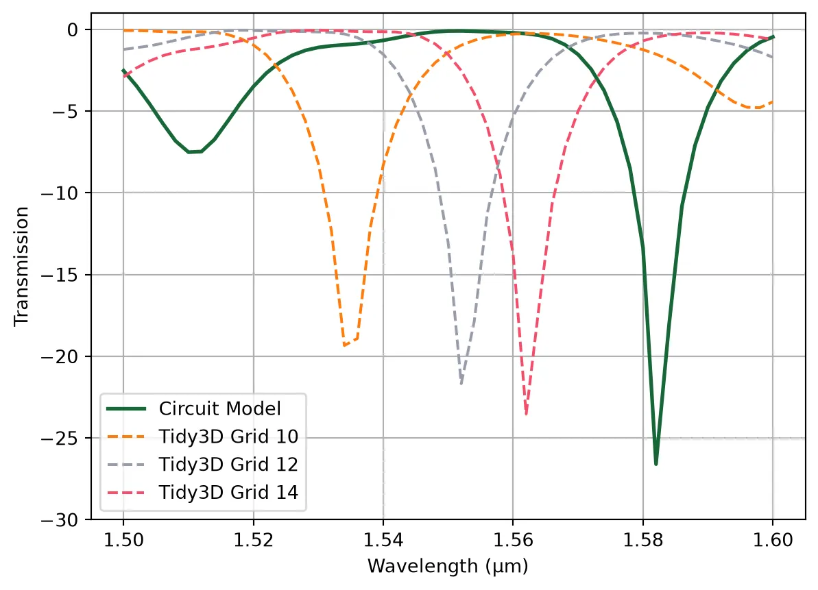
Finally, we compare the transmission spectra obtained from the circuit model and the full Tidy3D simulations. All results are plotted in dB scale.
Due to the extreme physical size of the spiral structure, achieving high accuracy with full FDTD simulation is not practically feasible—especially with limited computational resources. However, the plot below demonstrates that as we increase the mesh refinement (grid 10 → 12 → 14), the Tidy3D results progressively converge toward the circuit model prediction. This highlights the efficiency and reliability of the compact circuit modeling approach for large photonic components.
# Define the file names and grid labels for each Tidy3D resultsnp_files = {    "Grid 10": "misc/s_matrix_tidy3D_spiral_grid10.s2p",    "Grid 12": "misc/s_matrix_tidy3D_spiral_grid12.s2p",    "Grid 14": "misc/s_matrix_tidy3D_spiral_grid14.s2p",}
# Plot Circuit Model resultplt.plot(    wavelengths,    10 * np.log10(np.abs(s_matrix_circuit[("P0@0", "P1@0")]) ** 2),    label="Circuit Model",    linewidth=2,)
# Plot each Tidy3D-based resultfor label, file in snp_files.items():    # Load the S-matrix from the Touchstone file    s_matrix = pf.SMatrix.load_snp(file)
    # Wrap in a DataModel    data_model = pf.DataModel(s_matrix)
    # Add and activate the model on the spiral component    spiral.add_model(data_model, label)    spiral.activate_model(label)
    # Get S-matrix at the given frequencies    s_matrix_data = spiral.s_matrix(freqs, model_kwargs={"inputs": ["P0"]})
    # Plot transmission from P0 to P1    plt.plot(        wavelengths,        10 * np.log10(np.abs(s_matrix_data[("P0@0", "P1@0")]) ** 2),        label=f"Tidy3D {label}",        linestyle="--",    )
# Finalize the plotplt.xlabel("Wavelength (µm)")plt.ylabel("Transmission")plt.ylim(-30, 1)plt.legend()plt.grid(True)plt.show()