Analytic Bragg Grating Model

Download notebook (.zip)

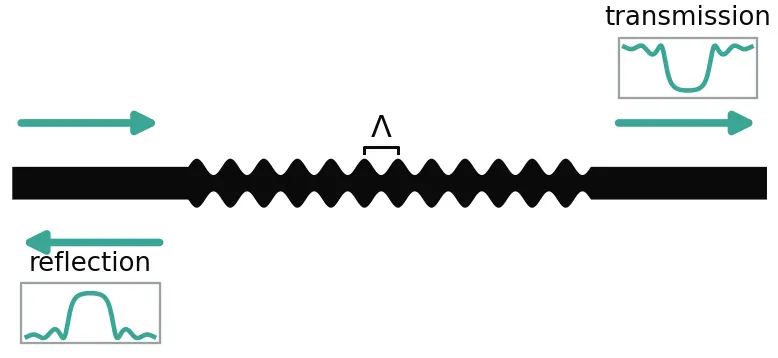
A waveguide Bragg grating (WBG) is a waveguide whose effective index is modulated periodically along its length, usually by corrugating the sidewalls. Light near the Bragg wavelength is reflected back into the input waveguide and the rest is transmitted. WBGs serve as on-chip mirrors for lasers and Fabry-Perot cavities, as notch and band-pass filters, and, when the period is chirped, as dispersive delay lines.

BraggGratingModel computes the full 2-port S matrix of a grating, reflection and transmission with their phase, from coupled-mode theory [1]. The grating can be uniform or vary along its length: the coupling strength can be apodized, the period can be chirped, and discrete phase shifts can be inserted. Propagation loss and waveguide dispersion are included.

This guide derives the model and computes its coupling coefficient from a single mode solve of the waveguide, using first-order perturbation theory for a moving boundary [2]. The grating is a silicon strip whose sidewalls follow a sinusoid, drawn as a parametric component that carries the model. One FDTD simulation of that layout serves as a benchmark, and the model is then used to design uniform, apodized, phase-shifted, and chirped gratings and a Fabry-Perot cavity built from two gratings.

References

1. Erdogan, Turan. “Fiber grating spectra.” Journal of Lightwave Technology 1997 15 (8), 1277-1294, doi: 10.1109/50.618322.
2. Johnson, Steven G., et al. “Perturbation theory for Maxwell’s equations with shifting material boundaries.” Physical Review E 2002 65 (6), 066611, doi: 10.1103/PhysRevE.65.066611.
3. Wang, Xu, et al. “Precise control of the coupling coefficient through destructive interference in silicon waveguide Bragg gratings.” Optics Letters 2014 39 (19), 5519-5522, doi: 10.1364/OL.39.005519.

Coupled-Mode Theory

A periodic perturbation of the waveguide couples the forward-propagating mode, with slowly varying amplitude $A(z)$, to the backward-propagating mode $B(z)$. The coupling accumulates only when the two modes stay in phase with the $m$-th harmonic of the perturbation, $2\beta = 2m\pi/\Lambda$, where $\Lambda$ is the grating period and $\beta = 2\pi n_\mathrm{eff}/\lambda$ is the propagation constant. This phase-matching condition defines the Bragg wavelength

$$\lambda_B = \frac{2 n_\mathrm{eff} \Lambda}{m}.$$

Away from $\lambda_B$ the phase mismatch is measured by the detuning

$$\hat\sigma = \beta - \frac{m\pi}{\Lambda},$$

and the two amplitudes obey the coupled-mode equations [1]

$$\frac{\mathrm{d}A}{\mathrm{d}z} = i\hat\sigma A + i\kappa B, \qquad \frac{\mathrm{d}B}{\mathrm{d}z} = -i\hat\sigma B - i\kappa^{*} A,$$

where the coupling coefficient $\kappa$ (in μm⁻¹) is the field amplitude scattered from one mode into the other per unit length.

For a uniform grating of length $L$ these linear equations have a closed-form solution. With $\gamma = \sqrt{\lvert\kappa\rvert^2 - \hat\sigma^2}$, the field reflection and transmission are

$$r = \frac{i\kappa^{*}\sinh(\gamma L)}{\gamma\cosh(\gamma L) + i\hat\sigma\sinh(\gamma L)}, \qquad t = \frac{\gamma}{\gamma\cosh(\gamma L) + i\hat\sigma\sinh(\gamma L)}.$$

Inside the stop band, $\lvert\hat\sigma\rvert < \lvert\kappa\rvert$, $\gamma$ is real and the field decays exponentially into the grating. Outside it, $\gamma$ is imaginary, the solution oscillates, and the reflection spectrum shows side lobes.

Two results of this solution guide every design below. At the Bragg wavelength ($\hat\sigma = 0$) the peak power reflectivity is

$$R_\mathrm{max} = \tanh^2(\kappa L),$$

so the product $\kappa L$ alone sets the strength of the mirror. The reflection band extends to the first zeros of $r$, where $\gamma L = i\pi$, that is $\hat\sigma^2 = \kappa^2 + (\pi/L)^2$. Differentiating $\beta$ gives $\mathrm{d}\hat\sigma/\mathrm{d}\lambda = -2\pi n_g/\lambda^2$, where $n_g$ is the group index, so the null-to-null bandwidth is

$$\Delta\lambda = \frac{\lambda_B^2}{\pi n_g L}\sqrt{(\kappa L)^2 + \pi^2}.$$

Short, weak gratings are limited by their length, $\Delta\lambda \approx \lambda_B^2/(n_g L)$, and long, strong gratings by their coupling, $\Delta\lambda \approx \lambda_B^2 \kappa/(\pi n_g)$.

A grating whose $\kappa$ or $\Lambda$ changes along $z$ is divided into num_sections uniform sections. Each section is solved with the expressions above and the section S matrices are cascaded. A uniform grating is exact with any number of sections, so the section count only has to resolve the variation of the apodization or the chirp. The default is the smaller of num_periods and 400.

Setup

import matplotlib.pyplot as plt
import numpy as np
import photonforge as pf
import tidy3d as td

# Start the LiveViewer used to display layouts
viewer = pf.live_viewer.LiveViewer()

LiveViewer started at http://127.0.0.1:43355. Call its 'stop()' method to free the port.

The default technology provides a 220 nm silicon strip waveguide in oxide (port spec "Strip", 500 nm wide). The grating sidewalls move by only 20 nm, so the layout polygons must follow the curve closely: pf.config.tolerance, the largest distance a polygon may deviate from the exact curve, is lowered from its 5 nm default to 1 nm. All indices are evaluated at $\lambda_0 = 1.55$ μm, and pf.C_0 is the speed of light in μm/s, so pf.C_0 / wavelength converts a wavelength in μm to a frequency in Hz.

# Set the default technology, which provides the 500 nm "Strip" port spec
tech = pf.basic_technology()
pf.config.default_technology = tech

# Set the maximal deviation of layout polygons from exact curves to 1 nm
pf.config.tolerance = 0.001

# We raise the Tidy3D logging level to reduce output noise from the FDTD simulation
# below. Warnings can flag real problems, so only suppress them once you have
# confirmed they are not relevant to your case.
td.config.logging.level = "ERROR"

lambda_0 = 1.55  # Design wavelength (μm)
f_ref = pf.C_0 / lambda_0  # Reference frequency of the effective and group indices (Hz)

Coupling Coefficient from the Mode Profile

This section computes $\kappa$ for a sinusoidal sidewall grating from the mode of the unperturbed 500 nm waveguide.

Each sidewall is displaced by $h(z) = a\sin(2\pi z/\Lambda)$, with $a = 20$ nm. Only the $e^{i2\pi z/\Lambda}$ component of the displacement, of amplitude $h_1 = a/2$, couples the forward mode to the backward mode at first order. In coupled-mode theory the coupling is the overlap of the permittivity change with the fields of the two modes, $\kappa = (\omega\varepsilon_0/4P)\iint \Delta\varepsilon_1\,\mathbf{E}_f\cdot\mathbf{E}_b^{*}\,\mathrm{d}A$, where $P$ is the mode power. For a moving boundary between high-contrast materials this overlap is ill-defined, because the field component normal to the sidewall jumps by $\varepsilon_\mathrm{Si}/\varepsilon_\mathrm{SiO_2} \approx 5.8$ across it. Johnson et al. [2] resolved this by writing the first-order change only in terms of field components that are continuous at the boundary, the tangential $\mathbf{E}_\parallel$ and the normal $D_\perp = \varepsilon E_\perp$. For the two sidewalls of the strip this gives

$$\kappa = \frac{\omega\varepsilon_0}{4P}\,2 h_1 \int_0^{t}\left[\Delta\varepsilon\,\mathbf{E}_{\parallel,f}\cdot\mathbf{E}_{\parallel,b}^{*} - \Delta\!\left(\varepsilon^{-1}\right) D_{\perp,f}\,D_{\perp,b}^{*}\right]\mathrm{d}z',$$

where the integral runs over the height $t$ of one sidewall, $\Delta\varepsilon = \varepsilon_\mathrm{Si} - \varepsilon_\mathrm{SiO_2}$ and $\Delta(\varepsilon^{-1}) = \varepsilon_\mathrm{Si}^{-1} - \varepsilon_\mathrm{SiO_2}^{-1}$ (relative permittivities).

The backward mode has the same transverse fields as the forward mode and the opposite longitudinal field. With $x$ along the propagation, $y$ normal to the sidewall and $z'$ vertical, $\mathbf{E}_\parallel = (E_x, E_{z'})$ and $D_\perp = D_y$, so

$$\mathbf{E}_{\parallel,f}\cdot\mathbf{E}_{\parallel,b}^{*} = \lvert E_{z'}\rvert^2 - \lvert E_x\rvert^2, \qquad D_{\perp,f}\,D_{\perp,b}^{*} = \lvert D_y\rvert^2.$$

The same integral with $\lvert E_{z'}\rvert^2 + \lvert E_x\rvert^2$ gives the change of $\beta$ when the waveguide widens, $\mathrm{d}\beta/\mathrm{d}w$ (each sidewall moves by $\mathrm{d}w/2$). The usual effective-index estimate, $\kappa = \pi\,\delta n/\lambda$ with $\delta n = (\mathrm{d}n_\mathrm{eff}/\mathrm{d}w)\,2a$, is therefore the right formula with the wrong sign on the longitudinal term. In a high-contrast strip, the longitudinal field at the sidewall is strong, so the effective-index estimate overestimates $\kappa$.

The integral needs the fields at the sidewall itself. The mode solver smooths the permittivity over the interface cell, so each continuous component is extrapolated to the sidewall with a cubic fit from each side, skipping two cells next to the interface, and the two sides are averaged. The first cell solves the mode and its power:

# Solve the fundamental mode of the Strip port with a fine mesh near the sidewall
mode = pf.port_modes(
    "Strip", [f_ref], mesh_refinement=80, verbose=False, show_progress=False
)

# Field components of the mode on its cross-section grid
components = ("Ex", "Ey", "Ez", "Hy", "Hz")
fields = {c: getattr(mode.data, c).isel(x=0, f=0, mode_index=0) for c in components}
y = (
    fields["Ey"].coords["y"].values
)  # Lateral grid coordinates, normal to the sidewall (μm)
z = fields["Ey"].coords["z"].values  # Vertical grid coordinates (μm)

# Area element of each grid cell (μm²)
area = np.gradient(y)[:, None] * np.gradient(z)[None, :]

# Power flow density along the propagation direction, (E x H*) . x
poynting = fields["Ey"].values * np.conj(fields["Hz"].values)
poynting -= fields["Ez"].values * np.conj(fields["Hy"].values)

# Mode power P (W)
power = 0.5 * np.real(np.sum(poynting * area))

# Relative permittivities of silicon and oxide in basic_technology at f_ref
eps_si = td.material_library["cSi"]["Li1993_293K"].eps_model(f_ref).real
eps_ox = td.material_library["SiO2"]["Palik_LowLoss"].eps_model(f_ref).real
print(f"eps_Si = {eps_si:.3f}, eps_SiO2 = {eps_ox:.3f}, mode power = {power:.3f} W")

eps_Si = 12.076, eps_SiO2 = 2.087, mode power = 1.000 W

The second cell evaluates the continuous components at the sidewall, checks the forward overlap against $\mathrm{d}n_\mathrm{eff}/\mathrm{d}w$ from two more mode solves, and computes $\kappa$ from the backward overlap:

width = 0.5  # Core width of the Strip port spec (μm)
amplitude = 0.02  # Sidewall displacement amplitude a (μm)
edge = width / 2  # Sidewall position along y (μm)
cell = np.diff(y).min()  # Smallest mode-solver cell size (μm)

# Fit windows inside and outside the core, two cells away from the sidewall
inside = (y > edge - 0.03) & (y < edge - 2 * cell)
outside = (y > edge + 2 * cell) & (y < edge + 0.03)

def at_sidewall(component, z_value, window):
    # Field component along y at height z_value
    values = fields[component].sel(z=z_value, method="nearest").values
    # Cubic fit in the window, evaluated at the sidewall
    return np.polyval(np.polyfit(y[window] - edge, values[window], 3), 0.0)

# Sidewall heights for the integral, 5 nm away from the core corners
z_wall = z[(z > 0.005) & (z < 0.215)]

# Tangential fields at the sidewall, averaged over both sides
e_x = (
    np.array(
        [
            at_sidewall("Ex", zi, inside) + at_sidewall("Ex", zi, outside)
            for zi in z_wall
        ]
    )
    / 2
)
e_z = (
    np.array(
        [
            at_sidewall("Ez", zi, inside) + at_sidewall("Ez", zi, outside)
            for zi in z_wall
        ]
    )
    / 2
)

# Normal displacement field D_y at the sidewall, averaged over both sides
d_y = (
    np.array(
        [
            eps_si * at_sidewall("Ey", zi, inside)
            + eps_ox * at_sidewall("Ey", zi, outside)
            for zi in z_wall
        ]
    )
    / 2
)

d_eps = eps_si - eps_ox  # Permittivity contrast across the sidewall
d_inv = 1 / eps_si - 1 / eps_ox  # Inverse-permittivity contrast across the sidewall
prefactor = (
    2 * np.pi * f_ref * td.constants.EPSILON_0 / (4 * power)
)  # Prefactor ω ε0 / (4P)
dz = np.gradient(z_wall)  # Integration step along the sidewall height (μm)

# Forward-forward overlap integral, which gives d(beta)/dw
forward = np.sum(
    (d_eps * (np.abs(e_z) ** 2 + np.abs(e_x) ** 2) - d_inv * np.abs(d_y) ** 2) * dz
)

# Slope dn_eff/dw from the forward overlap (1/μm)
dn_dw = prefactor * forward * lambda_0 / (2 * np.pi)

# Effective indices of 490 nm and 510 nm strips for a finite-difference slope
n_eff_of = {}
for w in (width - 0.01, width + 0.01):
    # Copy of the Strip spec with core width w
    spec = tech.ports["Strip"].copy()
    spec.path_profiles = [(w, 0.0, "WG_CORE"), (2.5, 0.0, "WG_CLAD")]
    # Mode solve of the modified spec, on the same fine mesh
    solved = pf.port_modes(
        spec, [f_ref], mesh_refinement=80, verbose=False, show_progress=False
    )
    n_eff_of[w] = float(solved.data.n_eff.isel(mode_index=0).values[0])

# Finite-difference slope dn_eff/dw (1/μm)
dn_dw_modes = (n_eff_of[width + 0.01] - n_eff_of[width - 0.01]) / 0.02
print(
    f"dn_eff/dw: {dn_dw:.3f} 1/μm from the overlap, {dn_dw_modes:.3f} 1/μm from mode solves"
)

# Forward-backward overlap integral, with the longitudinal term reversed
backward = np.sum(
    (d_eps * (np.abs(e_z) ** 2 - np.abs(e_x) ** 2) - d_inv * np.abs(d_y) ** 2) * dz
)

# Coupling coefficient: first harmonic a/2 of the displacement on two sidewalls (1/μm)
kappa = abs(prefactor * 2 * (amplitude / 2) * backward)

# Effective-index estimate π δn / λ with δn = (dn_eff/dw) 2a (1/μm)
kappa_index = np.pi * dn_dw_modes * 2 * amplitude / lambda_0
print(f"kappa = {kappa:.4f} 1/μm (effective-index estimate {kappa_index:.4f} 1/μm)")

dn_eff/dw: 1.546 1/μm from the overlap, 1.582 1/μm from mode solves
kappa = 0.0694 1/μm (effective-index estimate 0.1283 1/μm)

The forward overlap reproduces the $\mathrm{d}n_\mathrm{eff}/\mathrm{d}w$ of the mode solver to a few percent (the corners, left out of the integral, account for most of the difference), which shows that the fields are evaluated correctly at the sidewall. The effective-index estimate is about twice the coupling coefficient because it counts the longitudinal field with the wrong sign. Applied to the air-clad square-corrugation gratings of Wang et al. [3], the same calculation gives 0.036 μm⁻¹ and 0.072 μm⁻¹ for 10 nm and 20 nm corrugations, where their FDTD band-structure simulations report 0.037 μm⁻¹ and 0.069 μm⁻¹.

Sinusoidal Grating Layout

The parametric component below draws the grating from the path profiles of its port spec: the core width follows $w + 2a\sin(2\pi z/\Lambda)$, and every other profile, here the cladding, is drawn at constant width. pf.Path.segment takes the width as a pair of expressions in the normalized path coordinate $u \in [0, 1]$, the width and its derivative with respect to $u$. With a whole number of periods, both ends have the width of the port spec, so detect_ports finds the two ports.

The component carries a BraggGratingModel with the same period and number of periods. Its effective and group indices come from a mode solve of the port spec, whose width is the mean width of the grating, and its coupling coefficient is the value computed above.

@pf.parametric_component
def sinusoidal_grating(
    *,
    port_spec="Strip",
    period=0.316,
    num_periods=100,
    amplitude=0.02,
    coupling_coefficient=kappa,
):
    # Port spec from the default technology when given by name
    if isinstance(port_spec, str):
        port_spec = pf.config.default_technology.ports[port_spec]

    profiles = (
        port_spec.path_profiles_list()
    )  # (width, offset, layer) of each spec profile
    core_layer = min(profiles)[2]  # Layer of the narrowest profile, the core
    length = num_periods * period  # Grating length (μm)

    component = pf.Component("SINUSOIDAL_GRATING")
    for w, g, layer in profiles:
        if layer == core_layer:
            k = (
                2 * np.pi * num_periods
            )  # Angular spatial frequency in the path coordinate u
            # Core width w + 2a sin(k u) and its derivative with respect to u
            width_spec = (
                f"{w} + {2 * amplitude} * sin({k} * u)",
                f"{2 * amplitude * k} * cos({k} * u)",
            )
            # Core path, with about 32 boundary evaluations per period
            path = pf.Path((0, g), w).segment(
                (length, g), width_spec, min_evals=32 * num_periods
            )
            component.add(layer, path)
        else:
            # Constant-width profile, here the cladding
            component.add(layer, pf.Path((0, g), w).segment((length, g)))

    # Ports at both ends, where the core has the width of the port spec
    component.add_port(component.detect_ports())

    # Effective and group indices of the unperturbed waveguide, which has the mean grating width
    data = pf.port_modes(
        port_spec, [f_ref], group_index=True, verbose=False, show_progress=False
    ).data

    # Bragg model with the same period and number of periods as the layout
    model = pf.BraggGratingModel(
        period=period,
        num_periods=num_periods,
        coupling_coefficient=coupling_coefficient,
        n_eff=float(data.n_eff.isel(mode_index=0).values[0]),
        n_group=float(data.n_group.isel(mode_index=0).values[0]),
        reference_frequency=f_ref,
    )
    component.add_model(model, "Bragg")
    return component

# Short grating for display
grating = sinusoidal_grating(num_periods=20)
viewer(grating)

FDTD Benchmark

This section compares the model, with the coupling coefficient from the mode profile, against an FDTD simulation of the 50-period layout. The port symmetry halves the number of simulations, because the grating is mirror symmetric between its two ports.

The sidewall moves by only 20 nm, so the FDTD mesh must resolve that motion. A mesh override over the band that each sidewall sweeps sets 2 nm cells along $y$, across the sidewall, and 10 nm cells along $x$ and $z$, which resolve the sinusoid along the propagation direction and the core height. The rest of the domain uses 12 cells per wavelength. A coarser mesh across the sidewall averages the wobble away and underestimates $\kappa$, and a coarser mesh along $x$ or $z$ also shifts the Bragg wavelength.

# Grating with 50 periods for the benchmark
benchmark = sinusoidal_grating(num_periods=50)

thickness = 0.22  # Core thickness of basic_technology (μm)
band = (
    2 * amplitude + 0.02
)  # Width of the band each sidewall sweeps, with 10 nm margins (μm)

# Mesh overrides over each sidewall band: 2 nm cells along y, 10 nm cells along x and z
override = [
    td.MeshOverrideStructure(
        geometry=td.Box(
            center=(0, side * edge, thickness / 2),
            size=(td.inf, band, thickness + 0.04),
        ),
        dl=(0.01, 0.002, 0.01),
    )
    for side in (-1, 1)
]

# Base grid of 12 steps per wavelength, with the sidewall overrides
grid = td.GridSpec.auto(
    min_steps_per_wvl=12, wavelength=lambda_0, override_structures=override
)

# FDTD model with the mirror symmetry between the two ports
fdtd_model = pf.Tidy3DModel(port_symmetries=[("P1", "P0")], grid_spec=grid)

# Add the FDTD model to the grating, which also makes it the active model
benchmark.add_model(fdtd_model, "FDTD")

wavelengths_fdtd = np.linspace(1.45, 1.65, 401)  # Benchmark wavelengths (μm)

# S matrix of the grating from FDTD
s_fdtd = benchmark.s_matrix(pf.C_0 / wavelengths_fdtd)

# Bragg model as the active model again, for the comparison and the rest of the guide
benchmark.activate_model("Bragg")

Uploading task 'P0@0…'
Starting task 'P0@0': https://tidy3d.simulation.cloud/workbench?taskId=fdve-c56d9a67-9129-40d8-9765-27426ac7b5b0
Downloading data from 'P0@0'…

BraggGratingModel(period=0.316, num_periods=50, coupling_coefficient=np.float64(0.06941622650267192), n_eff=2.438925944215924, n_group=4.177737048234647, reference_frequency=193414489032258.06, order=1, loss=0.0, apodization='uniform', apodization_parameter=3.0, phase_shifts=(), num_sections=None, ports=None)

The coupling coefficient that the FDTD spectrum implies follows from its peak reflectivity, $\kappa = \operatorname{artanh}\sqrt{R_\mathrm{max}}/L$:

# S matrix of the same grating from the Bragg model
s_model = benchmark.s_matrix(pf.C_0 / wavelengths_fdtd)

# Reflected power from FDTD and from the model
r_fdtd = np.abs(s_fdtd[("P0@0", "P0@0")]) ** 2
r_model = np.abs(s_model[("P0@0", "P0@0")]) ** 2

# Length of the benchmark grating (μm)
length_50 = 50 * benchmark.active_model.parametric_kwargs["period"]

# Coupling coefficient implied by the FDTD peak reflectivity (1/μm)
kappa_fdtd = np.arctanh(np.sqrt(r_fdtd.max())) / length_50
print(f"kappa: {kappa:.4f} 1/μm from the mode profile, {kappa_fdtd:.4f} 1/μm from FDTD")
print(
    f"Peak wavelength: {wavelengths_fdtd[r_model.argmax()] * 1e3:.1f} nm (model), "
    f"{wavelengths_fdtd[r_fdtd.argmax()] * 1e3:.1f} nm (FDTD)"
)

fig, ax = plt.subplots(figsize=(7, 3.5))
ax.plot(wavelengths_fdtd * 1e3, r_fdtd, "k", lw=3, alpha=0.35, label="FDTD")
ax.plot(wavelengths_fdtd * 1e3, r_model, label="BraggGratingModel")
ax.set_xlim(1500, 1590)
ax.set_xlabel("Wavelength (nm)")
ax.set_ylabel("Reflection")
ax.legend()
ax.grid(alpha=0.3)
plt.show()

kappa: 0.0694 1/μm from the mode profile, 0.0686 1/μm from FDTD
Peak wavelength: 1545.0 nm (model), 1544.5 nm (FDTD)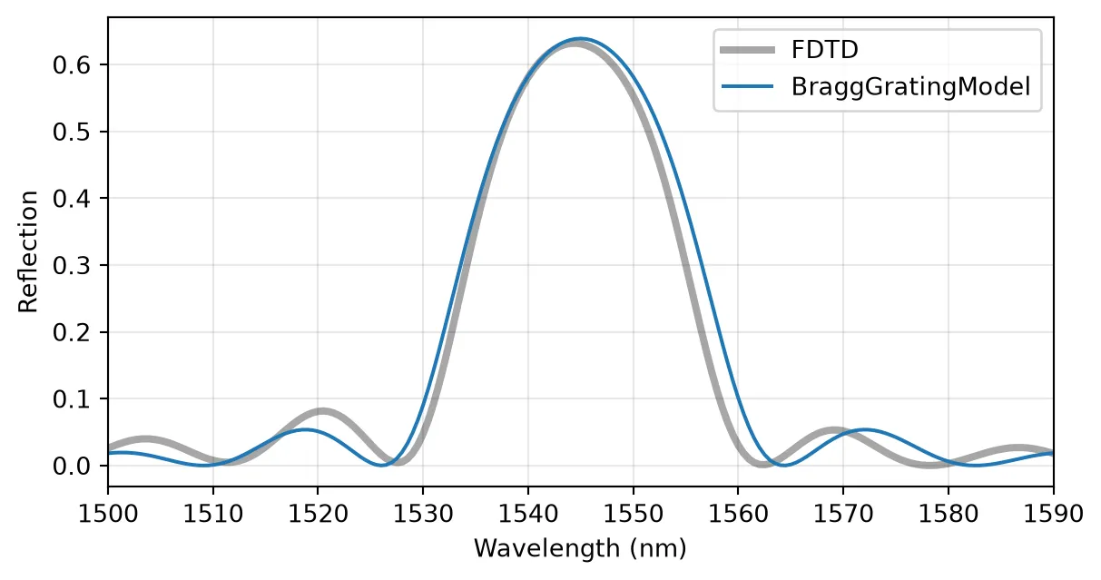

Uniform Grating

A 100-period grating from the same component, about 32 μm long, gives a strong reflector. The S matrix keys are (input, output) pairs of port@mode, so ("P0@0", "P0@0") is the reflection seen from P0 and ("P0@0", "P1@0") the transmission.

In a dispersive waveguide the Bragg wavelength is where the Bragg condition holds at its own wavelength, $\lambda_B = 2 n_\mathrm{eff}(\lambda_B)\Lambda/m$. The method bragg_wavelength() solves this condition for the mean period. With the first-order dispersion used here, $n_\mathrm{eff}(\lambda) = n_g + (n_{\mathrm{eff},0} - n_g)\lambda/\lambda_0$, where $n_{\mathrm{eff},0}$ is the index at $\lambda_0$, the solution has the closed form

$$\lambda_B = \frac{2\Lambda n_g}{1 - 2\Lambda(n_{\mathrm{eff},0} - n_g)/\lambda_0}.$$

For an n_eff given as an Interpolator, the method finds the root numerically inside the sampled frequencies. The peak reflectivity $\tanh^2(\kappa L)$ and the null-to-null band are drawn for reference:

# Grating with 100 periods and its Bragg model
grating = sinusoidal_grating(num_periods=100)
model = grating.active_model

period = model.parametric_kwargs["period"]  # Grating period (μm)
n_eff = model.parametric_kwargs["n_eff"]  # Effective index at f_ref
n_group = model.parametric_kwargs["n_group"]  # Group index
length = 100 * period  # Grating length (μm)

# Bragg wavelength of the grating, solved with the dispersive effective index (μm)
lambda_b = model.bragg_wavelength()

wavelengths = np.linspace(1.515, 1.575, 2001)  # Wavelengths for the spectra (μm)
freqs = pf.C_0 / wavelengths  # Corresponding frequencies (Hz)

# Reflection and transmission of the grating
s = grating.s_matrix(freqs)
r = s[("P0@0", "P0@0")]
t = s[("P0@0", "P1@0")]

# Peak reflectivity of a uniform grating
r_max = np.tanh(kappa * length) ** 2

# Null-to-null bandwidth of a uniform grating (μm)
bandwidth = (
    lambda_b**2 / (np.pi * n_group * length) * np.sqrt((kappa * length) ** 2 + np.pi**2)
)
print(f"Bragg wavelength = {lambda_b * 1e3:.2f} nm, grating length = {length:.1f} μm")
print(
    f"kappa L = {kappa * length:.2f}, R_max = {r_max:.4f}, bandwidth = {bandwidth * 1e3:.2f} nm"
)

fig, ax = plt.subplots(figsize=(7, 3.5))
ax.plot(wavelengths * 1e3, np.abs(r) ** 2, label="Reflection")
ax.plot(wavelengths * 1e3, np.abs(t) ** 2, label="Transmission")
ax.axhline(r_max, color="k", ls=":", lw=1)
for band_edge in (lambda_b - bandwidth / 2, lambda_b + bandwidth / 2):
    ax.axvline(band_edge * 1e3, color="k", ls=":", lw=1)
ax.set_xlabel("Wavelength (nm)")
ax.set_ylabel("Power")
ax.legend()
ax.grid(alpha=0.3)
plt.show()

Bragg wavelength = 1544.97 nm, grating length = 31.6 μm
kappa L = 2.19, R_max = 0.9515, bandwidth = 22.05 nm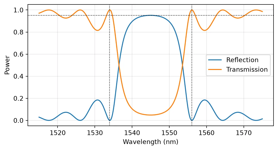

Grating Length

With $\kappa$ fixed by the sidewall amplitude, the number of periods sets $\kappa L$. A short grating is a weak, broadband reflector whose bandwidth is set by its length. As the grating grows, the reflectivity saturates at 1 and the band narrows toward the coupling-limited width $\lambda_B^2\kappa/(\pi n_g)$:

fig, ax = plt.subplots(figsize=(7, 3.5))
for num_periods in (25, 50, 100, 200):
    # Reflection of a grating with num_periods periods
    s_n = sinusoidal_grating(num_periods=num_periods).s_matrix(freqs)
    # Grating strength κL
    kl = kappa * num_periods * period
    ax.plot(
        wavelengths * 1e3,
        np.abs(s_n[("P0@0", "P0@0")]) ** 2,
        label=f"N = {num_periods}, κL = {kl:.1f}",
    )
ax.set_xlabel("Wavelength (nm)")
ax.set_ylabel("Reflection")
ax.legend(fontsize=8)
ax.grid(alpha=0.3)
plt.show()

# Coupling-limited bandwidth λ_B² κ / (π n_g)
print(
    f"Coupling-limited bandwidth: {lambda_b**2 * kappa / (np.pi * n_group) * 1e3:.2f} nm"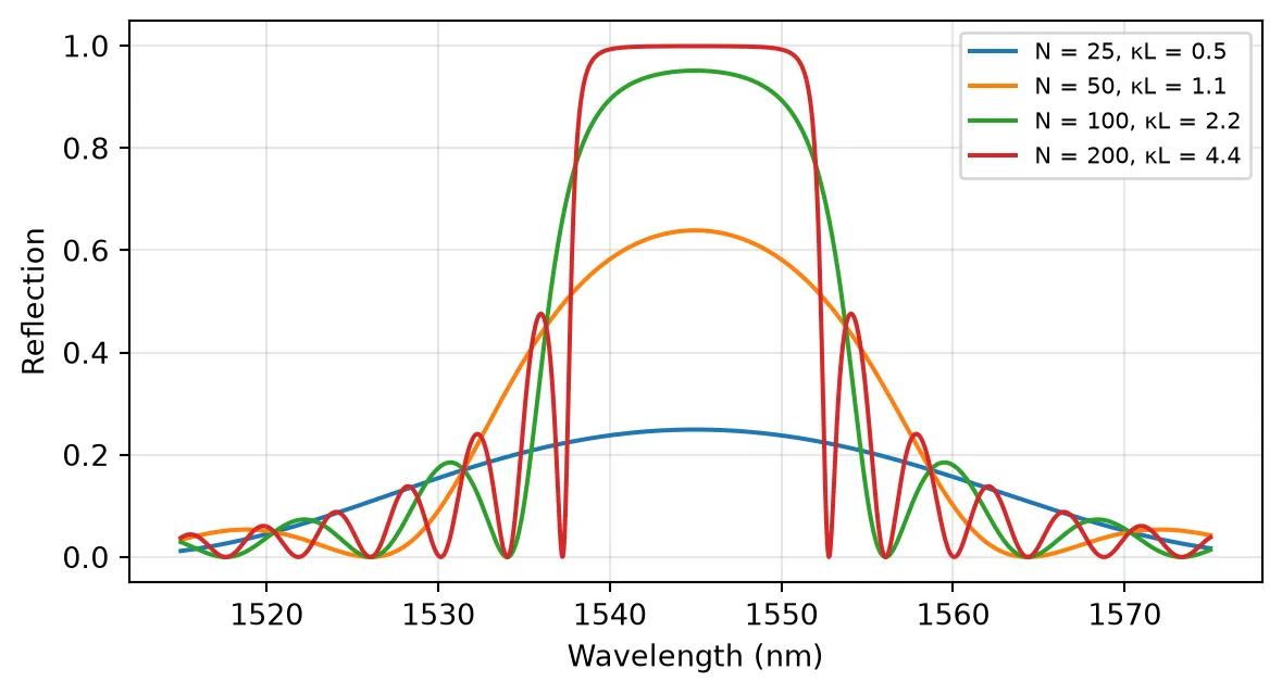
)

Coupling-limited bandwidth: 12.62 nm

Group Index and Bandwidth

Every spectral width in the model scales as $1/n_g$ through $\mathrm{d}\hat\sigma/\mathrm{d}\lambda$. Without n_group, the model uses a constant n_eff, which is equivalent to $n_g = n_\mathrm{eff}$, and all widths come out $n_g/n_\mathrm{eff}$ times too wide. For a silicon strip this factor is about 1.7. For dispersion beyond first order, n_eff also accepts an Interpolator over frequency.

# Same grating without n_group, so the effective index is constant
no_dispersion = pf.BraggGratingModel(
    period=period, num_periods=100, coupling_coefficient=kappa, n_eff=n_eff
)

# Reflection of the grating without dispersion
s_nd = no_dispersion.black_box_component(port_spec="Strip").s_matrix(freqs)

fig, ax = plt.subplots(figsize=(7, 3.5))
ax.plot(wavelengths * 1e3, np.abs(r) ** 2, label="n_group from the mode solver")
ax.plot(wavelengths * 1e3, np.abs(s_nd[("P0@0", "P0@0")]) ** 2, label="n_group not set")
ax.set_xlabel("Wavelength (nm)")
ax.set_ylabel("Reflection")
ax.legend()
ax.grid(alpha=0.3)
plt.show()

# Ratio by which widths grow when n_group is not set
print(f"n_group / n_eff = {n_group / n_eff:.2f}")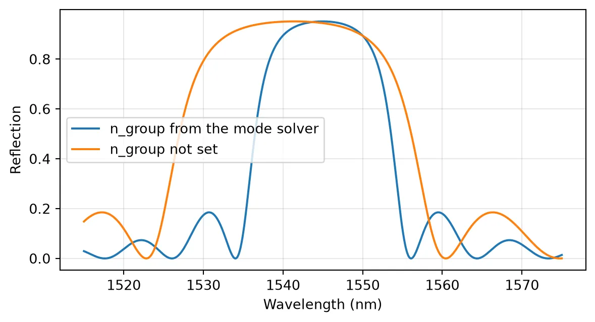

n_group / n_eff = 1.71

Apodization

For a weak grating, the reflection spectrum is approximately the Fourier transform of $\kappa(z)$. The abrupt start and end of a uniform grating therefore produce sinc-like side lobes, which cause crosstalk into neighboring channels when the grating is used as a filter. Tapering $\kappa(z)$ smoothly to zero at both ends suppresses them. For the sinusoidal grating, $\kappa$ is proportional to the sidewall amplitude, so apodization means a position-dependent amplitude. The mean width stays $w$, so to first order the average index, and with it the local Bragg wavelength, does not change along the grating.

The apodization argument scales $\kappa$ along the grating with a named window ("uniform", "gaussian", "raised-cosine", "blackman"), a sampled array, or an expression string in the normalized position $u = z/L$. apodization_parameter sets the width of the "gaussian" and "raised-cosine" windows. To compare windows before drawing any layout, black_box_component wraps a model in a plain 2-port component.

The method sections() returns the per-section $\kappa$, period, and length, which shows the profile that is actually simulated. The grating here has 200 periods ($\kappa L \approx 4.4$):

wavelengths_wide = np.linspace(1.49, 1.60, 3001)  # Wider wavelength range (μm)
freqs_wide = pf.C_0 / wavelengths_wide  # Corresponding frequencies (Hz)

fig, axes = plt.subplots(1, 2, figsize=(10, 3.5))
for apodization in ("uniform", "gaussian", "raised-cosine", "blackman", "sin(pi*u)"):
    # 200-period grating with the given apodization window
    apodized = pf.BraggGratingModel(
        period=period,
        num_periods=200,
        coupling_coefficient=kappa,
        n_eff=n_eff,
        n_group=n_group,
        reference_frequency=f_ref,
        apodization=apodization,
    )
    # Coupling coefficient and length of each section
    kappa_z, _, section_length = apodized.sections()
    # Position of each section centre along the grating (μm)
    position = np.cumsum(section_length) - section_length / 2

    # Uniform in gray, so the apodized curves stand out
    style = {"color": "0.6"} if apodization == "uniform" else {}
    axes[0].plot(position, np.abs(kappa_z), lw=1.2, label=apodization, **style)

    # Reflection in dB
    s_a = apodized.black_box_component(port_spec="Strip").s_matrix(freqs_wide)
    r_db = 10 * np.log10(np.abs(s_a[("P0@0", "P0@0")]) ** 2 + 1e-12)
    axes[1].plot(wavelengths_wide * 1e3, r_db, lw=1, **style)

axes[0].set_xlabel("Position z (μm)")
axes[0].set_ylabel("κ (1/μm)")
axes[1].set_xlabel("Wavelength (nm)")
axes[1].set_ylabel("Reflection (dB)")
axes[1].set_ylim(-70, 3)
for ax in axes:
    ax.grid(alpha=0.3)
axes[0].legend(fontsize=8)
fig.tight_layout()
plt.show()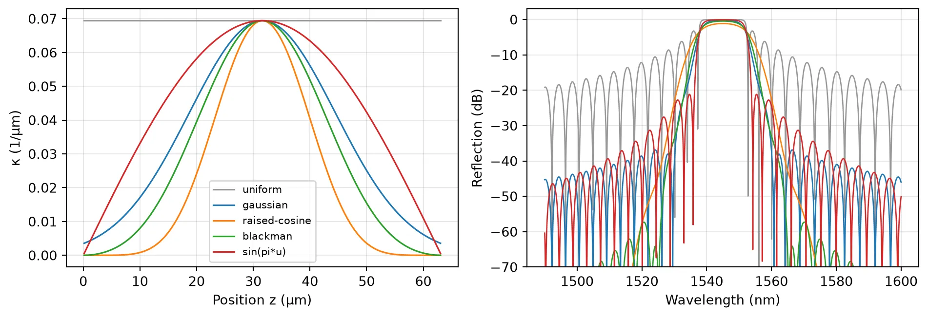

The tapered windows trade a slightly narrower top and a softer band edge for side lobes that are tens of dB lower.

Phase-Shifted Grating

phase_shifts takes (position, phase) pairs, with the position as the normalized coordinate $u$ and the phase in radians, and adds that phase to $\kappa$ from the given position onward. A shift of π at the center is a quarter-wave shift: it is the grating equivalent of inserting a spacer of length $\Lambda/2$, which adds a round-trip phase of $2\beta\Lambda/2 = \pi$ at $\lambda_B$. The two halves then act as two Bragg mirrors around a cavity that resonates exactly at $\lambda_B$, and a narrow transmission peak opens in the middle of the stop band.

Each half is a mirror of strength $\kappa L/2$ with power transmission $1 - \tanh^2(\kappa L/2) \approx 4 e^{-\kappa L}$, so the quality factor $Q$ grows as $e^{\kappa L}$ with the total length. Propagation loss caps it. A waveguide with power attenuation $\alpha$ (in 1/m) alone would have an intrinsic quality factor

$$Q_i = \frac{2\pi n_g}{\lambda \alpha},$$

and the peak transmission of a symmetric cavity falls as

$$T_\mathrm{peak} = \left(1 - \frac{Q}{Q_i}\right)^2.$$

The loss argument takes the propagation loss in dB/μm. The gratings below have 2 dB/cm of loss, a typical value for silicon strip waveguides:

loss = 2e-4  # Propagation loss: 2 dB/cm (dB/μm)
alpha = (
    loss * 1e6 * np.log(10) / 10
)  # Same loss as a power attenuation coefficient (1/m)

# Intrinsic quality factor set by the propagation loss
q_intrinsic = 2 * np.pi * n_group / (lambda_b * 1e-6 * alpha)
print(f"Intrinsic Q = {q_intrinsic:.3g}")

wavelengths_fine = np.linspace(
    lambda_b - 0.001, lambda_b + 0.001, 40001
)  # ±1 nm around λ_B (μm)
freqs_fine = pf.C_0 / wavelengths_fine  # Corresponding frequencies (Hz)
detuning_pm = (wavelengths_fine - lambda_b) * 1e6  # Detuning from λ_B (pm)

fig, ax = plt.subplots(figsize=(7, 3.5))
for num_periods in (180, 240, 300):
    # Lossy grating with a quarter-wave shift at its center
    shifted = pf.BraggGratingModel(
        period=period,
        num_periods=num_periods,
        coupling_coefficient=kappa,
        n_eff=n_eff,
        n_group=n_group,
        reference_frequency=f_ref,
        loss=loss,
        phase_shifts=[(0.5, np.pi)],
    )
    # Transmitted power around the resonance
    s_p = shifted.black_box_component(port_spec="Strip").s_matrix(freqs_fine)
    t_p = np.abs(s_p[("P0@0", "P1@0")]) ** 2

    # Wavelengths above half the peak transmission
    above = wavelengths_fine[t_p >= t_p.max() / 2]
    # Quality factor from the full width at half maximum
    q = lambda_b / (above.max() - above.min())
    print(
        f"N = {num_periods}: Q = {q:.3g}, peak T = {t_p.max():.3f}, "
        f"(1 - Q/Q_i)^2 = {(1 - q / q_intrinsic) ** 2:.3f}"
    )
    ax.plot(detuning_pm, t_p, label=f"N = {num_periods}")

ax.set_xlabel(r"Detuning from $\lambda_B$ (pm)")
ax.set_ylabel("Transmission")
ax.legend()
ax.grid(alpha=0.3)
plt.show()

Intrinsic Q = 3.69e+05
N = 180: Q = 3.02e+03, peak T = 0.983, (1 - Q/Q_i)^2 = 0.984
N = 240: Q = 1.14e+04, peak T = 0.939, (1 - Q/Q_i)^2 = 0.939
N = 300: Q = 3.93e+04, peak T = 0.798, (1 - Q/Q_i)^2 = 0.798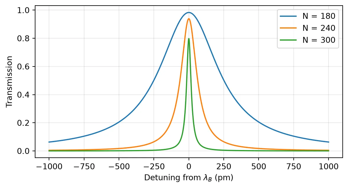

Each additional 60 periods multiplies $Q$ by about $e^{\kappa \cdot 60\Lambda} \approx 3.7$, while the peak transmission drops as $Q$ approaches $Q_i$. The design choice is therefore between linewidth and insertion loss, and the loss of the waveguide decides where the useful limit lies.

Chirped Grating

When the period varies along the grating, each wavelength is reflected where it is locally phase matched. The local Bragg condition $\beta(\lambda) = \pi/\Lambda(z)$ with a dispersive waveguide gives

$$\frac{\mathrm{d}\lambda_B}{\mathrm{d}\Lambda} = \frac{2 n_\mathrm{eff}^2}{n_g},$$

so a linear period change $\Delta\Lambda$ spreads the local Bragg wavelength over $\Delta\lambda_\mathrm{chirp} = 2 n_\mathrm{eff}^2 \Delta\Lambda / n_g$. When this span is much wider than the coupling-limited bandwidth, each wavelength is reflected from a well-defined position $z(\lambda)$ that moves linearly along the grating. The group delay $2 n_g z/c$ then changes linearly across the band, by up to $2 n_g L/c$ in total, which gives the dispersion

$$D \approx \frac{2 n_g L}{c\,\Delta\lambda_\mathrm{chirp}}.$$

Seen from the other end, the order of the wavelengths is reversed and $D$ changes sign.

The group delay is the frequency derivative of the reflection phase, $\tau = \mathrm{d}\phi/\mathrm{d}\omega$. The sign follows the PhotonForge convention, in which propagation over a length $L$ contributes $e^{+i\beta L}$.

A chirp is passed as period: an array, an Interpolator, or, as here, an expression string in $u$. This grating is 3000 periods (about 1 mm) long and its period changes linearly by 16 nm, from 308 nm to 324 nm, which spreads the reflection over about 46 nm, well beyond the 12.6 nm coupling-limited bandwidth. A gentle "raised-cosine" taper reduces the delay ripple caused by the abrupt grating ends, and the dispersion is fitted over the central 80% of the band:

chirp = 0.016  # Chirp coefficient: total change of the period along the grating (μm)
num_chirped = 3000  # Number of periods of the chirped grating

# Chirped grating with period Λ + chirp (u - 0.5) and a raised-cosine window
chirped = pf.BraggGratingModel(
    period=f"{period} + {chirp} * (u - 0.5)",
    num_periods=num_chirped,
    coupling_coefficient=kappa,
    n_eff=n_eff,
    n_group=n_group,
    reference_frequency=f_ref,
    apodization="raised-cosine",
    apodization_parameter=0.5,  # Window exponent 2a = 1, a single cosine
)
chirped_length = num_chirped * period  # Grating length (μm)

# Reflection seen from each end of the grating
s_c = chirped.black_box_component(port_spec="Strip").s_matrix(freqs_wide)
r_left = s_c[("P0@0", "P0@0")]
r_right = s_c[("P1@0", "P1@0")]

omega = 2 * np.pi * freqs_wide  # Angular frequencies (rad/s)

# Group delay from each end, dφ/dω of the unwrapped reflection phase (ps)
delay_left = np.gradient(np.unwrap(np.angle(r_left)), omega) * 1e12
delay_right = np.gradient(np.unwrap(np.angle(r_right)), omega) * 1e12

# Indices of the reflection band, where R > 0.5
band_index = np.flatnonzero(np.abs(r_left) ** 2 > 0.5)
trim = len(band_index) // 10  # Points dropped at each band edge (10% per side)
center = band_index[trim:-trim]  # Central 80% of the band
lambda_nm = wavelengths_wide * 1e3  # Wavelengths (nm)

# Dispersion from each end, slope of a linear fit to the delay (ps/nm)
d_left = np.polyfit(lambda_nm[center], delay_left[center], 1)[0]
d_right = np.polyfit(lambda_nm[center], delay_right[center], 1)[0]

chirp_span = 2 * n_eff**2 * chirp / n_group  # Span of local Bragg wavelengths (μm)
round_trip = (
    2 * n_group * chirped_length / pf.C_0 * 1e12
)  # Round-trip group delay 2 n_g L / c (ps)
print(f"Chirp span = {chirp_span * 1e3:.1f} nm, round-trip delay = {round_trip:.1f} ps")
print(f"Estimated D = {round_trip / (chirp_span * 1e3):.2f} ps/nm")
print(f"Fitted D = {d_left:.2f} ps/nm from P0, {d_right:.2f} ps/nm from P1")

fig, axes = plt.subplots(1, 2, figsize=(10, 3.5))
axes[0].plot(lambda_nm, np.abs(r_left) ** 2)
axes[0].set_ylabel("Reflection")
axes[1].plot(lambda_nm[band_index], delay_left[band_index], label="From P0")
axes[1].plot(lambda_nm[band_index], delay_right[band_index], label="From P1")
axes[1].set_ylabel("Group delay (ps)")
axes[1].legend()
for ax in axes:
    ax.set_xlabel("Wavelength (nm)")
    ax.grid(alpha=0.3)
fig.tight_layout()
plt.show()

Chirp span = 45.6 nm, round-trip delay = 26.4 ps
Estimated D = 0.58 ps/nm
Fitted D = 0.61 ps/nm from P0, -0.62 ps/nm from P1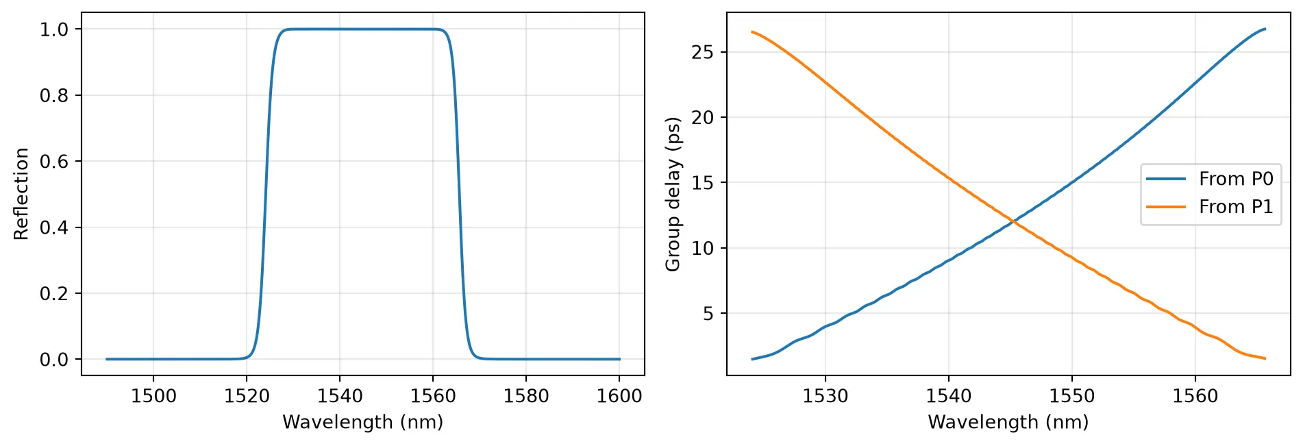

Fabry-Perot Cavity from Two Gratings

Because the model returns the complex reflection, including its phase at each end of the grating, it can be combined with other components in a CircuitModel. Here two 90-period sinusoidal gratings are joined by a straight waveguide, described by an AnalyticWaveguideModel with the same indices.

A spacer of $\Lambda/2$ is the layout form of the quarter-wave shift, so it reproduces the single 180-period grating with phase_shifts=[(0.5, np.pi)], which is drawn dashed for comparison. A longer spacer supports several cavity modes inside the stop band. Their spacing is set by the spacer plus the penetration of the field into both mirrors.

# Grating with 90 periods used as each cavity mirror
mirror = sinusoidal_grating(num_periods=90)

cavities = {}
for spacer in (period / 2, 50.0):
    cavity = pf.Component("BRAGG_CAVITY")

    # First mirror
    left = cavity.add_reference(mirror)

    # Straight spacer of the given length, with analytic propagation
    straight = pf.parametric.straight(
        port_spec="Strip",
        length=spacer,
        model=pf.AnalyticWaveguideModel(
            n_eff=n_eff, n_group=n_group, reference_frequency=f_ref
        ),
    )

    # Spacer connected to the first mirror, second mirror connected to the spacer
    middle = cavity.add_reference(straight).connect("P0", left["P1"])
    right = cavity.add_reference(mirror).connect("P0", middle["P1"])

    # Outer ports of the two mirrors as the cavity ports
    cavity.add_port([left["P0"], right["P1"]])

    # Circuit model that cascades the mirrors and the spacer
    cavity.add_model(pf.CircuitModel(), "Circuit")
    cavities[spacer] = cavity

viewer(cavities[50.0])

LayoutSchematic

# Single lossless grating with a quarter-wave shift, for comparison
shifted = pf.BraggGratingModel(
    period=period,
    num_periods=180,
    coupling_coefficient=kappa,
    n_eff=n_eff,
    n_group=n_group,
    reference_frequency=f_ref,
    phase_shifts=[(0.5, np.pi)],
)

# Transmission of the phase-shifted grating
s_ref = shifted.black_box_component(port_spec="Strip").s_matrix(freqs)

fig, ax = plt.subplots(figsize=(7, 3.5))
for spacer, cavity in cavities.items():
    # Transmission of each cavity
    s_cav = cavity.s_matrix(freqs)
    ax.plot(
        wavelengths * 1e3,
        np.abs(s_cav[("P0@0", "P1@0")]) ** 2,
        label=f"Spacer {spacer:.3g} μm",
    )
ax.plot(
    wavelengths * 1e3,
    np.abs(s_ref[("P0@0", "P1@0")]) ** 2,
    "k--",
    lw=1,
    label="phase_shifts=[(0.5, π)]",
)
ax.set_xlabel("Wavelength (nm)")
ax.set_ylabel("Transmission")
ax.legend(fontsize=8)
ax.grid(alpha=0.3)
plt.show()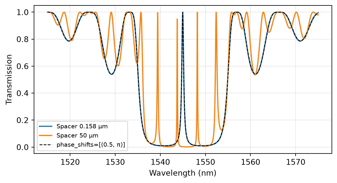

Abstract Component

For schematic-level work without a layout, abstract.bragg_grating wraps the model in a ready-made component with the same arguments:

# Abstract Bragg grating with the parameters of the 100-period layout
abstract_grating = pf.abstract.bragg_grating(
    period=period,
    num_periods=100,
    coupling_coefficient=kappa,
    n_eff=n_eff,
    n_group=n_group,
    reference_frequency=f_ref,
)
viewer(abstract_grating)

Summary

• BraggGratingModel solves the coupled-mode equations section by section and returns the complex reflection and transmission of a 2-port grating.
• The peak reflectivity is $\tanh^2(\kappa L)$ and the null-to-null bandwidth is $\lambda_B^2\sqrt{(\kappa L)^2 + \pi^2}/(\pi n_g L)$. Set n_group and reference_frequency, or pass n_eff as an Interpolator, so that the bandwidths use the group index.
• For sidewall gratings, $\kappa$ follows from one mode solve through the first-order moving-boundary overlap of Johnson et al. [2], written with the continuous field components $\mathbf{E}_\parallel$ and $D_\perp$. The longitudinal field enters with opposite signs for the forward and backward modes, which is why the effective-index estimate overestimates $\kappa$ in high-contrast waveguides.
• A sinusoidal sidewall is drawn with a width expression in pf.Path.segment; its FDTD benchmark needs a mesh that resolves the sidewall motion.
• apodization shapes $\kappa$ along the grating to suppress side lobes, phase_shifts inserts discrete shifts such as the quarter-wave shift, and period accepts a profile in $u$ for chirped gratings. sections() shows the discretized profile.
• loss sets the propagation loss in dB/μm, which limits the $Q$ and the peak transmission of phase-shifted gratings.
• The model can be attached to a grating layout inside a parametric component, combined with other components in a CircuitModel, or used through pf.abstract.bragg_grating.