Data Model

Download notebook (.zip)

The data model is used when the S parameters for a component are available as value arrays, for example, loaded from a Touchstone (snp) file. This type of model allows the use of data imported from alternative sources and, in particular, experimental data to be used for simulation.

import numpy as np
import photonforge as pf
from matplotlib import pyplot as plt

pf.config.default_technology = pf.basic_technology()

Sample Data Generation

For practical reasons, we’ll first create a Touchstone file with data from a Tidy3D model simulation, instead of running an actual experiment. The following component is not practical, but it is a small example that provides an interesting S parameter curve.

component = pf.Component("MAIN")

component.add(
    "WG_CORE",
    pf.Path((0, -2.5), 0.5)
    .segment((0, -2))
    .segment((0, -1.5), 0.2)
    .segment((0, 1.5))
    .segment((0, 2), 0.5)
    .segment((0, 2.5)),
    "SLAB",
    *[pf.Rectangle(center=(0, i * 0.4), size=(2, 0.25)) for i in range(-4, 5)]
)

component.add("WG_CLAD", pf.envelope(component, 1, trim_y_min=True, trim_y_max=True))

component.add_port(component.detect_ports())

component.add_model(pf.Tidy3DModel(port_symmetries=[("P1", "P0")]), "Tidy3D")

component

The S matrix values will be computed using 21 equally-spaced points in wavelength domain:

s_matrix = component.s_matrix(pf.C_0 / np.linspace(1.3, 1.7, 21))

plt.plot(pf.C_0 / s_matrix.frequencies, np.abs(s_matrix["P0@0", "P0@0"]), label="Reflection")
plt.plot(pf.C_0 / s_matrix.frequencies, np.abs(s_matrix["P0@0", "P1@0"]), label="Transmission")
plt.xlabel("Wavelength (μm)")
_ = plt.legend()

Uploading task 'P0@0…'
Starting task 'P0@0': https://tidy3d.simulation.cloud/workbench?taskId=fdve-bc18a650-9f78-4ead-b631-a261f62eebe6
Downloading data from 'P0@0'…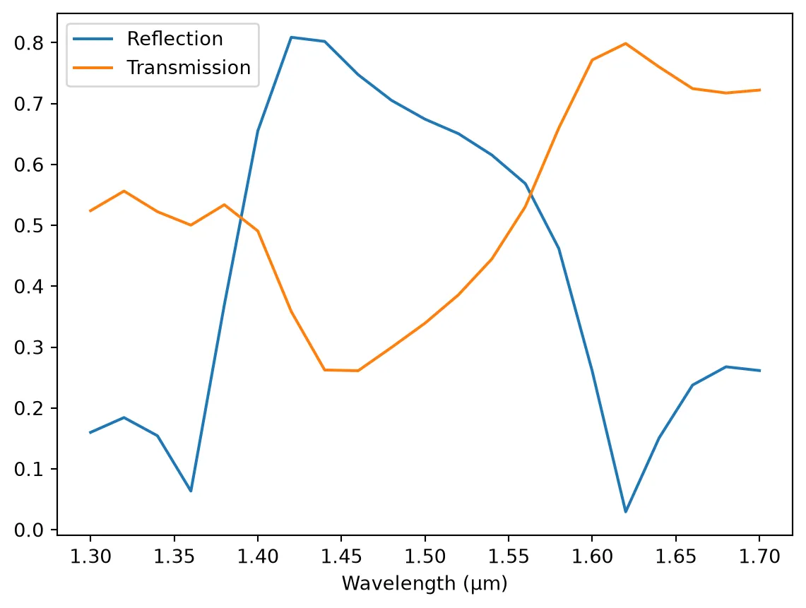

The data is written to a Touchstone file to be loaded as if it were experimental data.

_ = s_matrix.write_snp("data.s2p")

Loading S Matrix Data

Loading Touchstone files can be done with the load_snp function or the SMatrix.load_snp method. The former returns an array with the S matrix values and another with their corresponding frequencies, and the latter creates an S matrix object directly and is usually easier to use.

loaded_s_matrix = pf.SMatrix.load_snp("data.s2p")

data_model = pf.DataModel(loaded_s_matrix, interpolation_method="linear")

The data model can be used just as any other model to generate S parameters for the component they are assigned to. The only condition that must be respected is that the number of ports/modes of the component must match the model’s.

For example, we can create a black-box components and use our experimental data model to include the component in larger systems with circuit models.

black_box = pf.Component("BB")

black_box.add_port(pf.Port((0, 0), 0, "Strip"), "P0")
black_box.add_port(pf.Port((1, 0), 180, "Rib"), "P1")

black_box.add_model(data_model, "Data")

black_box

freqs = pf.C_0 / np.linspace(1.3, 1.7, 101)
s_data = black_box.s_matrix(freqs)

plt.plot(pf.C_0 / s_matrix.frequencies, np.abs(s_matrix["P0@0", "P0@0"]), "o")
plt.plot(pf.C_0 / s_data.frequencies, np.abs(s_data["P0@0", "P0@0"]))
plt.xlabel("Wavelength (μm)")
_ = plt.ylabel("Reflection")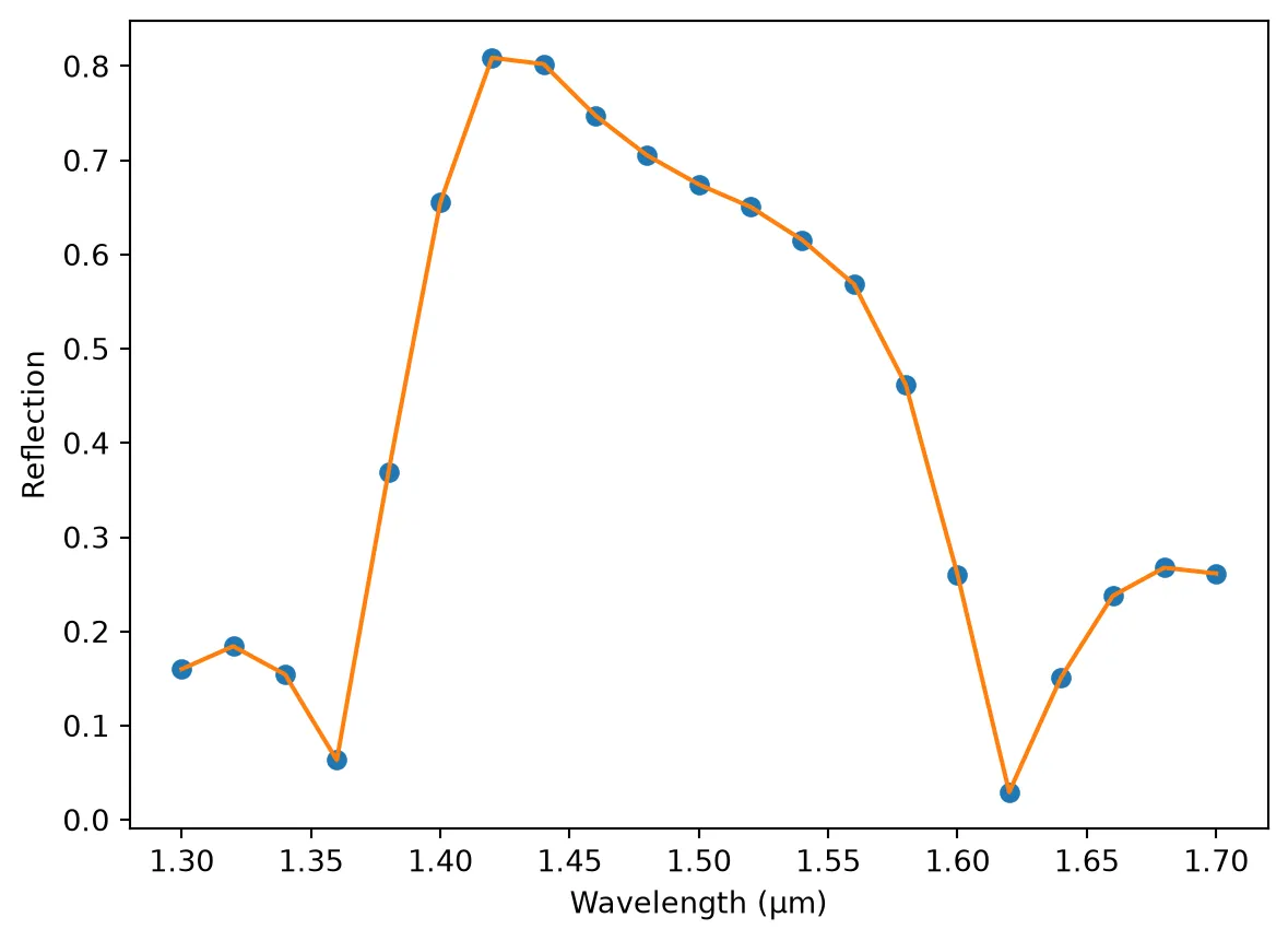

Interpolation

Note that the S matrix retrieved from the data model earlier used a different set of frequency points from the original. The data model computes the S parameters using linear interpolation by default, but that can be easily changed to a few other methods, documented in the data model constructor. Let’s use the "akima" method for a smoother interpolation:

model = pf.DataModel(loaded_s_matrix, interpolation_method="akima")

s_data = model.s_matrix(component, freqs)

plt.plot(pf.C_0 / s_matrix.frequencies, np.abs(s_matrix["P0@0", "P0@0"]), "o")
plt.plot(pf.C_0 / s_data.frequencies, np.abs(s_data["P0@0", "P0@0"]))
plt.xlabel("Wavelength (μm)")
_ = plt.ylabel("Reflection")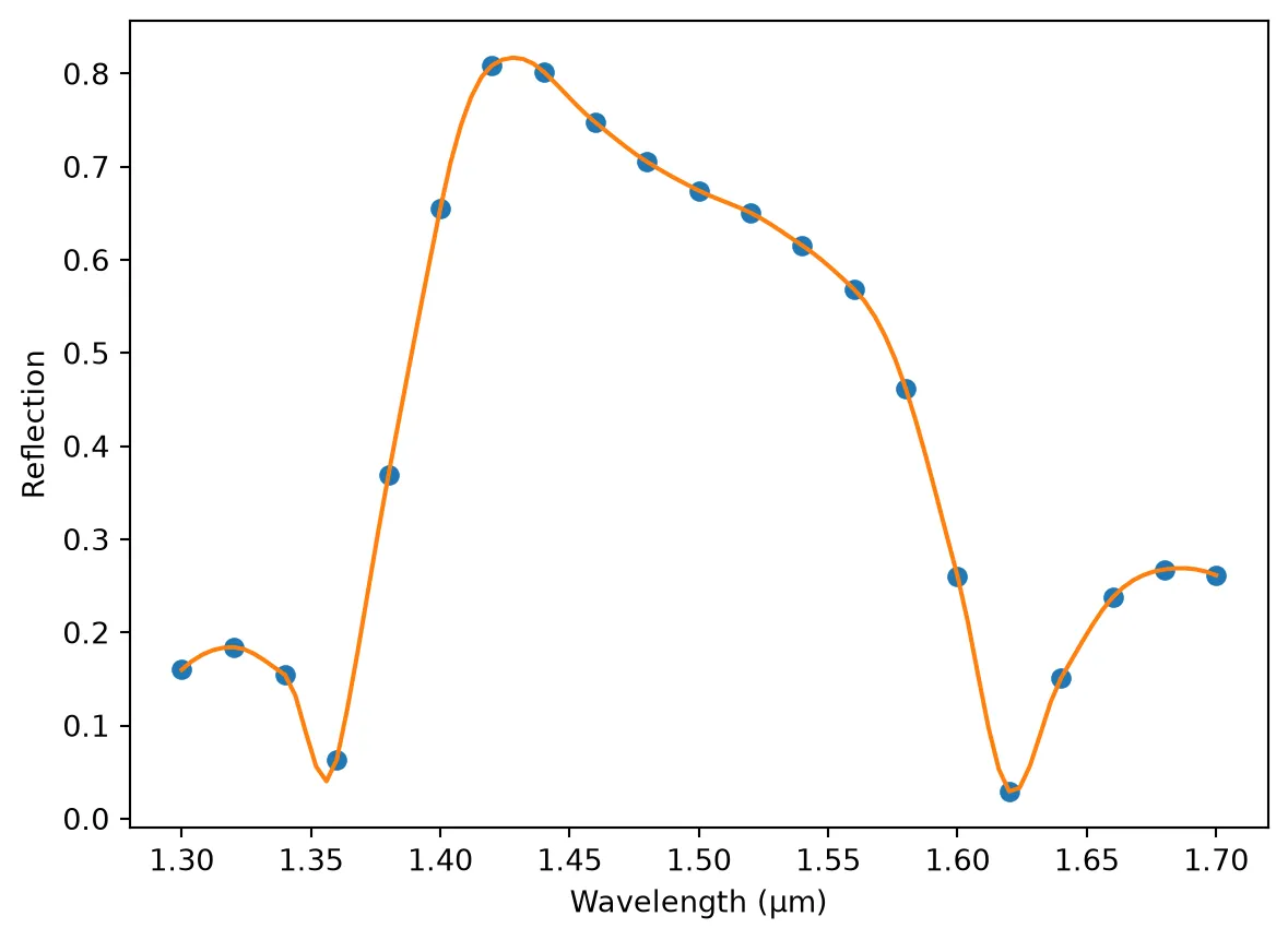

By default, the interpolation is applied to the magnitude and phases independently. It is also possible to interpolate using the real and imaginary components of the S parameters, but that usually leads to large phase jumps.

Data model from an S-matrix array

You can also create a DataModel directly from s_array and frequencies.

In the usual S-parameter convention, s_ij means input at port j and output at port i. In PhotonForge, the dictionary key order uses (ports[i], ports[j]), and the array-to-dictionary conversion is:

s_dict[(ports[i], ports[j])] = s_array[:, j, i]

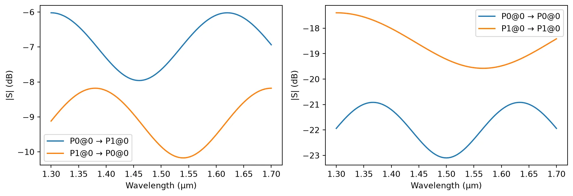
So when moving from matrix notation to the PhotonForge dictionary mapping, you should swap i and j in the array indexing. This is especially important for nonreciprocal devices, where forward and reverse transmission are different.

# Shape: (F, N, N) with N=2 ports
s_array = np.zeros((len(freqs), 2, 2), dtype=complex)
phi = np.linspace(0, np.pi, len(freqs))

# Add slight frequency-domain amplitude variation
amp_fwd = 0.45 + 0.05 * np.cos(2.5 * phi)
amp_rev = 0.35 + 0.04 * np.sin(2.5 * phi)

# Nonreciprocal transmission terms:
# Typical s_ij: input at j, output at i
# PhotonForge mapping: s_dict[(ports[i], ports[j])] = s_array[:, j, i]
s_array[:, 1, 0] = amp_fwd * np.exp(1j * phi)
s_array[:, 0, 1] = amp_rev * np.exp(-1.2j * phi)

# Small reflections with mild frequency variation
s_array[:, 0, 0] = 0.08 + 0.01 * np.sin(3 * phi)
s_array[:, 1, 1] = (0.12 + 0.015 * np.cos(1.5 * phi)) * np.exp(0.5j * phi)

data_model_from_array = pf.DataModel(
    s_array=s_array,
    frequencies=freqs,
    interpolation_method="linear",
)

black_box.add_model(data_model_from_array, "Array Data")

s_matrix_array = data_model_from_array.s_matrix(black_box, freqs)
_ = pf.plot_s_matrix(s_matrix_array, y="dB")