800G Coherent Transmitter Components

Download notebook (.zip)

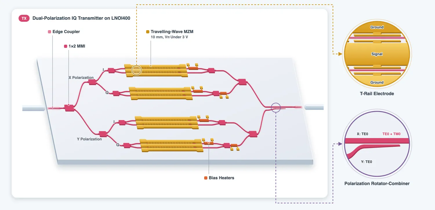
This page builds the component library of the transmitter chip on the Luxtelligence LNOI400 process [1]: the 1x2 multimode interference (MMI) splitter, the travelling-wave phase shifter that carries the data, the heater that sets the bias of each modulator, the polarization rotator-combiner (PRC) and the edge coupler. Each component gets a measured response, which the link page uses as its model.

The technology page introduced the process and the link budget. The transmitter is a dual-polarization IQ modulator: a 1x2 MMI splits the laser light between two IQ modulators, each IQ modulator is two Mach-Zehnder modulators (MZMs) nested in a third interferometer, and the PRC combines the two polarizations into one waveguide. The layout page assembles the components into the chip.

References

1. Luxtelligence LNOI400 process design kit and design manual, available from luxtelligence.ai/resources.
2. Kharel, Prashanta, et al. “Breaking voltage-bandwidth limits in integrated lithium niobate modulators using micro-structured electrodes.” Optica 2021 8 (3), 357-363, doi: 10.1364/OPTICA.416155.
3. Xu, Mengyue, et al. “Dual-polarization thin-film lithium niobate in-phase quadrature modulators for terabit-per-second transmission.” Optica 2022 9 (1), 61-62, doi: 10.1364/OPTICA.449691.
4. Gan, Ranfeng, et al. “Fabrication tolerant and broadband polarization splitter-rotator based on adiabatic mode evolution on thin-film lithium niobate.” Optics Letters 2022 47 (19), 5200-5203, doi: 10.1364/OL.471489.
5. Moretti, Paul, et al. “Temperature dependence of the dispersion relation of lithium niobate.” Journal of Applied Physics 2005 98 (3), 036101, doi: 10.1063/1.1988987.
6. Shin, Jaesang, et al. “Novel T-rail electrodes for substrate removed low-voltage high-speed GaAs/AlGaAs electrooptic modulators.” IEEE Transactions on Microwave Theory and Techniques 2005 53 (2), 636-643, doi: 10.1109/TMTT.2004.840735.
7. Behzadfar, S., F. Karami, P. Kulkarni, and S. Fathpour. “Ultimate performance of thin-film lithium niobate Mach-Zehnder modulators.” arXiv 2609.16379 (2026), arxiv.org/abs/2609.16379.

Three of the simulations on this page take hours of FDTD or EME, so their results are loaded from data files: coherent_trail_line.json, coherent_prc_coefficients.json, coherent_prc_delay.json and coherent_tx_edge_coupler.json. Each is preceded by the setup and followed by a commented cell with the code that produced it, which can be uncommented to run the simulation again or to try a different structure.

import json

import shapely

import luxtelligence_lnoi400_forge as lx
import matplotlib.pyplot as plt
import numpy as np
import photonforge as pf
import tidy3d as td
import tidy3d.web as web
from luxtelligence_lnoi400_forge import component as lxc

td.config.logging.level = "ERROR"

lda0 = 1.55  # Design wavelength (um)
f0 = pf.C_0 / lda0  # Design frequency (Hz); pf.C_0 is the speed of light in um/s
c0 = 299792458.0  # Speed of light in m/s, for the microwave arithmetic

tech = lx.lnoi400()
pf.config.default_technology = tech
viewer = pf.live_viewer.LiveViewer()

14:33:50 -03 WARNING: The material-library variant 'Palik_Lossless' is          
             deprecated and maps to 'Palik_LowLoss' because it contains a tiny  
             fitted loss despite its name. Use 'Palik_NoLoss' where available   
             for a zero-loss Palik model.                                       

LiveViewer started at http://127.0.0.1:36393. Call its 'stop()' method to free the port.

1x2 MMI

The 1x2 MMI splits the light into the two polarization branches, then into the two arms of every interferometer, and is used backwards as the combiner at each output. A transmitter path crosses seven of them, so their excess loss and their balance matter. The PDK provides an optimized 1x2 MMI for 1550 nm. The cell below attaches an FDTD model to it. One input is enough, because the other ports follow from reciprocity.

# FDTD model on the PDK cell, 12 mesh cells per wavelength
mmi = lxc.mmi1x2_optimized1550(
    technology=tech, model=pf.Tidy3DModel(grid_spec=12, verbose=False)
)
viewer(mmi)

wls = np.linspace(1.50, 1.60, 11)
s_mmi = mmi.s_matrix(pf.C_0 / wls, model_kwargs={"inputs": ["P0"]})

# The FDTD result becomes the model of the MMI: the paths from P0 to each output, and back by
# reciprocity. The reflections are left out (see below).
through = {k: v for k, v in s_mmi.elements.items() if k[0].startswith("P0") != k[1].startswith("P0")}
through |= {(b, a): v for (a, b), v in through.items()}
mmi_model = pf.DataModel(pf.SMatrix(s_mmi.frequencies, through), interpolation_method="linear")
# Use a constant matrix as time stepper: the MMI delays light by less than one time step of the link
mmi_model.time_stepper = pf.SMatrixTimeStepper(min_poles=0, max_poles=0, feedthrough=True, delays=0.0, passive=False)
mmi.add_model(mmi_model, "FDTD data")

# Power in each output and the reflection back into the input
t1 = np.abs(s_mmi[("P0@0", "P1@0")]) ** 2
t2 = np.abs(s_mmi[("P0@0", "P2@0")]) ** 2
r = np.abs(s_mmi[("P0@0", "P0@0")]) ** 2
excess = -10 * np.log10(t1 + t2)
print(f"excess loss at 1550 nm {np.interp(lda0, wls, excess):.3f} dB")
print(f"imbalance over the band below {np.max(np.abs(10 * np.log10(t2 / t1))):.3f} dB")
print(f"reflection below {10 * np.log10(r.max()):.1f} dB")

fig, ax = plt.subplots(1, 1, figsize=(5.5, 3.6))
ax.plot(wls * 1e3, excess)
ax.set_xlabel("wavelength (nm)")
ax.set_ylabel("excess loss (dB)")
ax.set_title("1x2 MMI")
plt.show()

excess loss at 1550 nm 0.094 dB
imbalance over the band below 0.000 dB
reflection below -43.6 dB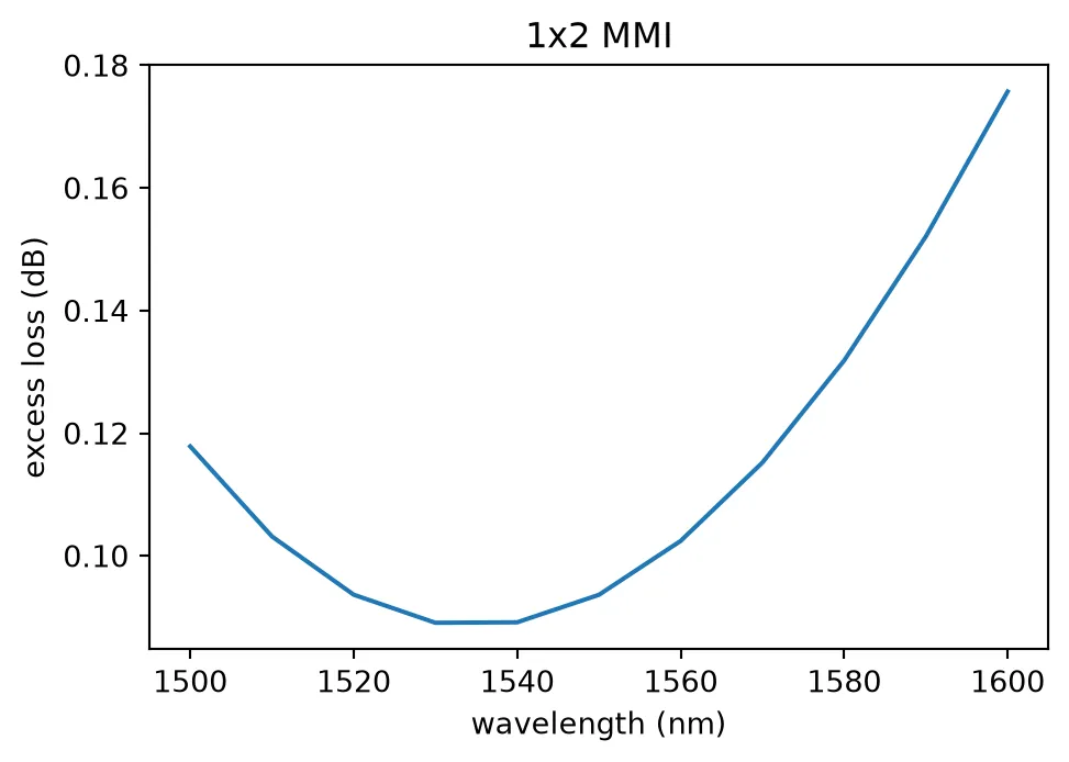

The MMI loses about 0.1 dB and splits evenly at every wavelength. The FDTD result is now the model of the MMI, a DataModel. Each MMI of the chip layout uses this model, and so does the link page.

The time stepper of the model is a constant matrix. The phase slope of the MMI is a delay of about 0.24 ps, less than the 2.08 ps time step of the link simulation. A pole fit cannot follow a delay that short while it stays causal and passive, and its result loses up to 1 dB. Over the 132 GHz of the signal the response is flat, so a constant matrix holds it exactly, less this sub-step delay.

Travelling-wave phase shifter

The data is written by the Pockels effect: a voltage $V$ across the lithium niobate film changes its extraordinary index, and a TE mode travelling along $x$ in an x-cut film sees that change. The index change of the mode per volt, $\partial n_\text{eff} / \partial V$, sets the voltage that shifts the phase by $\pi$ over a length $L$:

$$V_\pi L = \frac{\lambda}{2\,\partial n_\text{eff} / \partial V}.$$

An MZM driven push-pull has the field of one electrode gap in each arm with opposite signs, so the two arms move in opposite directions and their phase difference reaches $\pi$ at half the voltage of one arm. The product $V_\pi L$ quoted below is the push-pull value.

At 120 GBd the electrode cannot be a lumped capacitor: a 10 mm line is longer than the microwave wavelength at 60 GHz. It is a transmission line, a coplanar waveguide (CPW) with the optical arms in its two gaps, and the voltage travels along it with the light. The modulator works if three conditions hold together:

• Velocity match. The microwave index $n_\text{RF}$ must equal the optical group index $n_g$, so the light rides on the same part of the voltage wave along the whole line.
• Impedance match. The line impedance $Z_0$ must be 50 ohm, so the driver delivers its full voltage and nothing reflects from the termination.
• Low microwave loss. The voltage decays along the line by the conductor loss of the gold, which grows with $\sqrt{f}$, and by dielectric loss, which grows with $f$.

A plain CPW on thin-film lithium niobate has a microwave index well below the optical group index, because most of its field is in the oxide and the air. The PDK’s T-rail electrode adds a row of small T-shaped teeth along both edges of the gap [2]. The teeth add capacitance per unit length without adding the resistance a narrower gap would, which raises $n_\text{RF}$ toward $n_g$ and keeps the line loss low. The PDK provides the T-rail line as trail_cpw with the UniCPW-HS cross-section.

Half-wave voltage

The cell below solves the microwave mode of the CPW at a T-rail, with the optical arms in its gaps, and normalizes its field to one volt between signal and ground. The Pockels index change $\Delta n_e = -\tfrac{1}{2} n_e^3 r_{33} E_y$ is then written into the lithium niobate as a spatially varying index, and the optical arm is solved again at a few voltages. The slope of its effective index is $\partial n_\text{eff}/\partial V$.

# CPW cross-section at a T-rail: signal 27 um, gap 4 um, ground 183 um (the PDK UniCPW-HS line plus its rails)
cpw_rail = pf.cpw_spec(
    (21, 0),
    27.0,
    4.0,
    183.0,
    description="CPW at a rail",
    added_solver_modes=0,
    target_neff=2.2,
    technology=tech,
)
# Optical arm of the PDK modulator: a 2.5 um ridge on a 10 um slab
arm_spec = pf.PortSpec(
    description="PDK MZM arm",
    width=8.0,
    limits=(-1.5, 1.9),
    num_modes=1,
    target_neff=2.2,
    path_profiles=((2.5, 0, (2, 0)), (10.0, 0, (3, 0))),
)

# Arms centred in the two gaps
gw, go, _ = cpw_rail.path_profiles["gnd1"]
sw, _, _ = cpw_rail.path_profiles["signal"]
offset = (go - gw / 2 + sw / 2) / 2
gap = go - gw / 2 - sw / 2

opt = pf.port_modes(
    arm_spec, [f0], group_index=True, verbose=False, show_progress=False
)
n_group_arm = opt.data.n_group.values.ravel()[0]
print(f"optical arm: n_eff {opt.data.n_eff.values.ravel()[0]:.4f}  n_group {n_group_arm:.4f}")

# Microwave mode of the CPW with both arms, meshed inside the film as finely as the optical solve
mzm_spec = cpw_rail.combined_with(arm_spec, offset).combined_with(arm_spec, -offset)
dz = np.diff(opt.simulation.grid.boundaries.z).min()
ln_t = tech.parametric_kwargs["ln_thickness"]
rf = mzm_spec.to_tidy3d(frequencies=[1e9], mesh_refinement=25)
rf = rf.updated_copy(
    "simulation/grid_spec",
    override_structures=[
        td.MeshOverrideStructure(
            geometry=td.Box(center=(0, s * offset, ln_t / 2), size=(td.inf, gap, ln_t)),
            dl=(None, dz, dz),
        )
        for s in (-1, 1)
    ],
)
rf_data = pf.port_modes(rf, verbose=False, show_progress=False).data

# Field per volt: divide by the voltage between signal and ground
ic = cpw_rail.to_tidy3d_impedance_calculator()
v0 = ic.voltage_integral.compute_voltage(rf_data)
ey = (rf_data.Ey / v0).isel(f=0, mode_index=0, drop=True).abs
ey = ey.assign_coords(y=ey.y - offset)

optical arm: n_eff 1.8434  n_group 2.1794

# Lithium niobate indices at 1550 nm; the c axis is y, so n_e is the yy component
ln = td.material_library["LiNbO3"]["Zelmon1997"](optical_axis=1)
eps_o, eps_e, _ = (e.real for e in ln.eps_diagonal(f0))
n_e = eps_e**0.5
r33 = 30.9e-6  # Pockels coefficient (um/V)
dn_per_volt = -0.5 * n_e**3 * r33 * ey
eps_o_map = td.SpatialDataArray(
    np.full((1, 1, 1), eps_o), coords={"x": [0], "y": [0], "z": [0]}
)

# Re-solve the arm with the film index shifted by the field of each voltage
n_eff_v = []
volts = np.arange(5)
for v in volts:
    ln_v = td.CustomAnisotropicMedium(
        xx=td.CustomMedium(permittivity=eps_o_map, subpixel=True),
        yy=td.CustomMedium(permittivity=(n_e + v * dn_per_volt) ** 2, subpixel=True),
        zz=td.CustomMedium(permittivity=eps_o_map, subpixel=True),
    )
    s = pf.port_modes(
        arm_spec,
        [f0],
        technology=lx.lnoi400(ln=ln_v),
        verbose=False,
        show_progress=False,
    )
    n_eff_v.append(s.data.n_eff.isel(mode_index=0, f=0).item())

dn_dv = abs(n_eff_v[-1] - n_eff_v[0]) / (volts[-1] - volts[0])
vpil = lda0 / (2 * dn_dv) / 2  # push-pull, in V um
print(f"dn_eff/dV {dn_dv:.3e} per volt")
print(f"V_pi L push-pull {vpil * 1e-4:.2f} V cm")

dn_eff/dV 1.396e-05 per volt
V_pi L push-pull 2.78 V cm

The two fields that enter this number are plotted below, centred on one arm. The microwave field per volt fills the 4 um gap between the rail heads and is nearly uniform across the ridge, so most of the optical mode sees it. The cut through the middle of the film shows the overlap that sets $\partial n_\text{eff}/\partial V$: the optical intensity sits where the microwave field is strongest.

# Microwave field per volt and the optical mode of the arm, both centred on the arm
ey_map = ey.squeeze()
e_opt = opt.data.Ey.isel(f=0, mode_index=0).abs.squeeze()
z_rail = ln_t + tech.parametric_kwargs["tl_separation"]  # bottom of the gold
t_rail = tech.parametric_kwargs["tl_thickness"]

fig, ax = plt.subplots(1, 3, figsize=(17, 3.8), gridspec_kw={"width_ratios": [1.3, 1.3, 1]})
im = ax[0].pcolormesh(ey_map.y, ey_map.z, ey_map.T, shading="auto", cmap="magma")
fig.colorbar(im, ax=ax[0], label="microwave E_y per volt (1/um)")
im = ax[1].pcolormesh(e_opt.y, e_opt.z, e_opt.T, shading="auto", cmap="magma")
fig.colorbar(im, ax=ax[1], label="optical |E_y| (a.u.)")
for a, title in zip(ax[:2], ("microwave field at a rail", "optical mode of the arm")):
    # Rail heads on both sides of the gap, and the film outline
    for side in (-1, 1):
        y0 = side * gap / 2
        a.add_patch(plt.Rectangle((y0, z_rail), side * 3, t_rail, fc="none", ec="w", lw=1))
    a.plot([-4, 4], [0, 0], "w-", lw=0.6)
    a.plot([-4, 4], [ln_t, ln_t], "w--", lw=0.6)
    a.set_xlim(-4, 4)
    a.set_ylim(-1.0, 2.6)
    a.set_aspect("equal")
    a.set_xlabel("y (um)")
    a.set_ylabel("z (um)")
    a.set_title(title)

# Horizontal cut through the middle of the film
z_mid = ln_t / 2
rf_cut = ey_map.interp(z=z_mid)
opt_cut = (e_opt**2).interp(z=z_mid)
ax[2].plot(rf_cut.y, rf_cut / rf_cut.max(), label="microwave E_y")
ax[2].plot(opt_cut.y, opt_cut / opt_cut.max(), label="optical intensity")
ax[2].set_xlim(-4, 4)
ax[2].set_xlabel("y (um)")
ax[2].set_ylabel("normalized")
ax[2].set_title(f"cut at z = {z_mid:.1f} um")
ax[2].legend()
plt.show()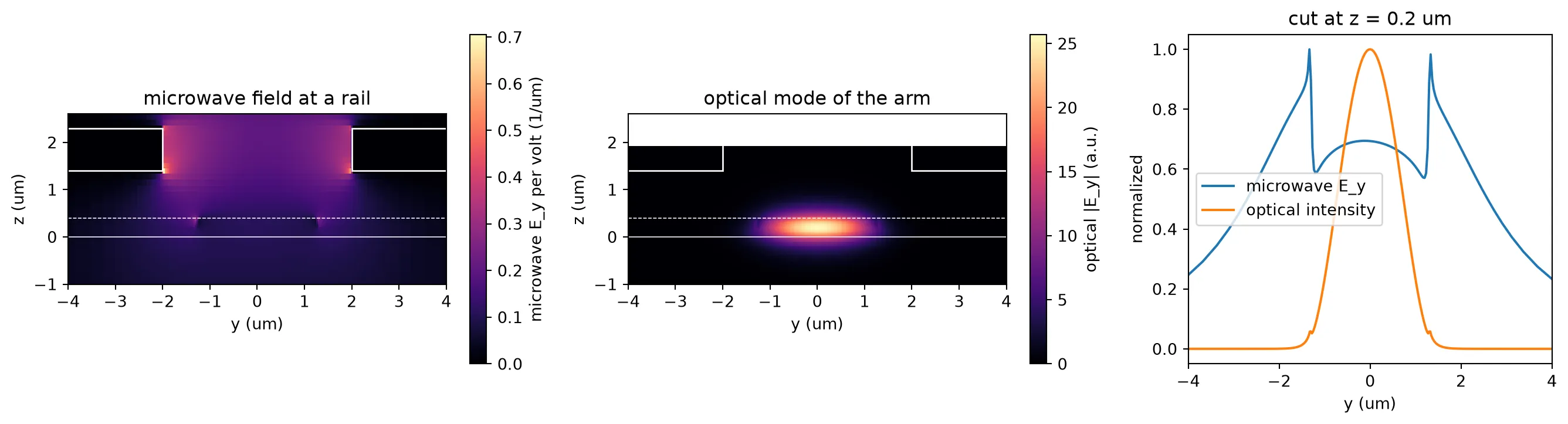

What this calculation assumes

The optical waveguide is the same all along the modulator, so its mode is exactly a 2D mode solution. The electrode is not: the T-rail line is periodic, and the microwave field the light sees changes along the propagation direction. The calculation above takes the field of an infinitely long rail, a 2D cross-section through a rail head. The exact field is a 3D quantity, which would need a 3D electrostatic or FDTD solution of a period of the electrode with the optical waveguide inside it.

The difference comes from the gaps between rail heads. Each period of the PDK line is 49.7 um long: a 44.7 um rail head and a 5 um spacing to the next. Under a head the electrodes are 4 um apart. In a spacing the heads are missing and the electrodes fall back toward the 10 um gap of the unloaded line, so the field across the waveguide drops there. The phase the light accumulates is the average of the index change along its path, so the effective $V_\pi L$ is

$$(V_\pi L)_\text{eff} = \frac{(V_\pi L)_\text{rail}}{f + (1 - f)\,\eta},$$

with $f$ the fraction of each period under a rail head, the duty cycle, and $\eta$ the field in a spacing relative to the field under a head. This is why T-rail designs keep the duty cycle high: Behzadfar et al. [7] hold it at 90 % and note that the modulating field is confined to the loaded rail gap, which makes $V_\pi$ a property of the rail gap and the duty cycle. Two bounds follow without a new simulation. With no field at all in the spacings, $\eta = 0$, the penalty is the duty cycle alone. If the field in a spacing were that of the unloaded 10 um gap, $\eta$ would be the ratio of the gaps, about 0.4. The fringing field of the neighbouring heads, which are only 5 um apart, fills part of each spacing, so the true $\eta$ lies above that.

# T-rail period of the PDK line (um): a 44.7 um rail head and a 5 um spacing
period = 49.7
duty = 44.7 / period  # Fraction of a period under a rail head
for label, eta in (("no field in the spacings", 0.0), ("unloaded 10 um gap in the spacings", gap / 10.0)):
    factor = 1 / (duty + (1 - duty) * eta)
    print(f"{label:36s} V_pi L {vpil * factor * 1e-4:.2f} V cm (+{100 * (factor - 1):.0f} %)")

# The value the rest of the series uses: the unloaded-gap estimate, the upper end of the likely range
vpil_eff = vpil / (duty + (1 - duty) * gap / 10.0)
print(f"V_pi L used from here on {vpil_eff * 1e-4:.2f} V cm")

no field in the spacings             V_pi L 3.09 V cm (+11 %)
unloaded 10 um gap in the spacings   V_pi L 2.95 V cm (+6 %)
V_pi L used from here on 2.95 V cm

The two limits give 3.09 V cm, with no field in the spacings, and 2.95 V cm, with the field of the unloaded gap. The fringing field of the rail heads puts the real value below 2.95 V cm, about 5 % above the rail value of 2.78 V cm. The rest of the series uses 2.95 V cm, the upper end of that likely range, so the modulators are not driven deeper than the real electrode allows: the length trade below and the drive voltages of the link page both start from it. A 3D simulation of one period of the electrode would replace this estimate with a computed value.

Microwave line

The microwave index, impedance and loss of the T-rail line come from a 3D FDTD simulation of the electrode. The simulated structure is a plain CPW feed, a section of 20 T-rail periods, and the feed again. The feeds are de-embedded with the impedance and index of the plain CPW from a mode solve, and what remains is the ABCD matrix of the T-rail section, which gives its propagation constant and its impedance at each frequency. The loss is taken from two T-rail sections, of 10 and of 20 periods, so the feed error cancels between them. Above 70 GHz a mode of the 1 mm simulation box crosses the CPW mode, so the high band was simulated again with a second port mode and a shorter section. The cell below builds the 20-period structure as it was simulated, and loads the extracted line parameters from coherent_trail_line.json.

# Plain CPW feed: the PDK UniCPW-HS line without rails, one wavelength at 10 GHz long
feed_spec = pf.cpw_spec(
    (21, 0),
    21.0,
    10.0,
    180.0,
    description="feed CPW",
    limits=(-500, 500),
    num_modes=1,
    target_neff=2.2,
    technology=tech,
)
l_feed = pf.snap_to_grid(0.01 * td.C_0 / 10e9)
feed = pf.parametric.straight(port_spec=feed_spec, length=l_feed, technology=tech)
loaded = lxc.trail_cpw(
    port_spec=feed_spec, length=20 * period, name="LOADED", technology=tech
)

# Feed, 20 T-rail periods, feed
trail_fdtd = pf.Component("TRAIL_FDTD", technology=tech)
r_in = trail_fdtd.add_reference(feed)
r_mid = trail_fdtd.add_reference(loaded).connect("E0", r_in["E1"])
r_out = trail_fdtd.add_reference(feed).connect("E0", r_mid["E1"])
trail_fdtd.add_port(r_in["E0"], "E0")
trail_fdtd.add_port(r_out["E1"], "E1")
trail_fdtd.add_model(
    pf.Tidy3DModel(
        boundary_spec=td.BoundarySpec(
            x=td.Boundary.pml(num_layers=30), y=td.Boundary.pml(), z=td.Boundary.pml()
        ),
        port_symmetries=[("E1", "E0")],
        verbose=False,
    ),
    "Tidy3D",
)
viewer(trail_fdtd)

LayoutSchematic

line = json.load(open("misc/coherent_trail_line.json"))
f_line = np.array(line["f_nz"]) * 1e-9
f_loss = np.array(line["f"]) * 1e-9
loss_fit = line["loss_fit"]  # alpha = a sqrt(f) + b f, f in GHz, alpha in dB/cm
n_rf, z0_line = line["N_RF"], line["Z0"]
print(f"microwave index {n_rf:.3f}, optical group index {line['n_g']:.3f}")
print(f"impedance {z0_line:.1f} ohm")
print(
    f"loss {loss_fit[0]:.3f} sqrt(f) + {loss_fit[1]:.4f} f dB/cm, "
    f"{loss_fit[0] * np.sqrt(60) + loss_fit[1] * 60:.2f} dB/cm at 60 GHz"
)

f_fit = np.linspace(1, 100, 200)
fig, ax = plt.subplots(1, 3, figsize=(15, 3.6))
ax[0].plot(f_line, line["n_rf"], "o-", label="T-rail line")
ax[0].axhline(line["n_g"], color="0.4", ls="--", label="optical group index")
ax[0].set_ylabel("index")
ax[0].legend()
ax[1].plot(f_line, line["z0"], "o-")
ax[1].axhline(50, color="0.4", ls="--")
ax[1].set_ylim(30, 80)
ax[1].set_ylabel("impedance (ohm)")
ax[2].plot(f_loss, line["alpha"], "o", label="FDTD")
ax[2].plot(f_fit, loss_fit[0] * np.sqrt(f_fit) + loss_fit[1] * f_fit, label="fit")
ax[2].set_ylabel("loss (dB/cm)")
ax[2].legend()
for a in ax:
    a.set_xlabel("frequency (GHz)")
plt.show()

microwave index 2.194, optical group index 2.181
impedance 50.6 ohm
loss 0.379 sqrt(f) + 0.0273 f dB/cm, 4.57 dB/cm at 60 GHz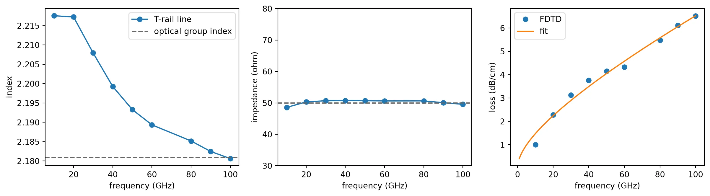

Why two sections of 10 and 20 periods, rather than one period

A single period is enough to find the microwave index and the impedance: its ABCD matrix gives the propagation constant through $\cosh(\gamma \Lambda) = (A + D)/2$, and the Bloch impedance follows from the same matrix. The loss is different. One 49.7 um period loses about 0.02 dB at 60 GHz, and the error left after the feeds are removed is of the same size: the transition from the plain feed to the first rail and the launch of the port mode are not described exactly by the mode solve of the plain line used to remove the feeds. A loss taken from one period is therefore mostly that error.

A longer section makes the loss larger than the error, and 20 periods also give the phase of the line ten times more room, which sharpens the index. The remaining error does not depend on the length of the section, so simulating two lengths removes it: the loss per unit length is $\alpha = 2\alpha_{20} - \alpha_{10}$, where $\alpha_N$ is the loss per unit length extracted from the $N$-period section. This is the two-line method of microwave metrology, and it matters here because the loss sets the bandwidth of the modulator.

The cell below is the code that produced coherent_trail_line.json, commented out because each FDTD run covers a 1 mm wide box around a 1 mm long electrode. Uncomment it to rerun the extraction, or change period, the rail geometry or the feed to study another electrode.

# # Two T-rail sections, 10 and 20 periods long, each between two plain CPW feeds
# f_rf = np.linspace(10e9, 60e9, 6)  # above ~70 GHz a box mode crosses the CPW: use 2 port modes there
# ms_feed, z_feed = pf.port_modes(feed_spec, f_rf, impedance=True, mesh_refinement=24, verbose=False)
# n_feed = np.asarray(ms_feed.data.n_complex.sel(mode_index=0)).ravel()
# z_feed = np.asarray(z_feed.sel(mode_index=0)).ravel()
# extracted = {}
# for n_periods in (10, 20):
#     length = n_periods * period
#     dut = pf.Component(f"TRAIL_{n_periods}", technology=tech)
#     a = dut.add_reference(feed)
#     b = dut.add_reference(lxc.trail_cpw(port_spec=feed_spec, length=length, technology=tech))
#     b.connect("E0", a["E1"])
#     c = dut.add_reference(feed).connect("E0", b["E1"])
#     dut.add_port(a["E0"], "E0")
#     dut.add_port(c["E1"], "E1")
#     dut.add_model(trail_fdtd.active_model, "Tidy3D")
#     s = dut.s_matrix(f_rf, model_kwargs={"inputs": ["E0@0"]})
#     # S parameters to the ABCD matrix of the whole structure (conjugate: microwave sign convention)
#     s11, s21 = np.conj(s[("E0@0", "E0@0")]), np.conj(s[("E0@0", "E1@0")])
#     n_rf_n, z0_n, alpha_n = [], [], []
#     for i, f in enumerate(f_rf):
#         d = 2 * s21[i]
#         total = np.array([
#             [((1 + s11[i]) * (1 - s11[i]) + s21[i] ** 2) / d, z_feed[i] * ((1 + s11[i]) ** 2 - s21[i] ** 2) / d],
#             [((1 - s11[i]) ** 2 - s21[i] ** 2) / (d * z_feed[i]), ((1 - s11[i]) * (1 + s11[i]) + s21[i] ** 2) / d],
#         ])
#         # Remove one feed on each side: the inverse of the feed's ABCD matrix
#         gl = 2 * np.pi * f / c0 * (n_feed.imag[i] + 1j * n_feed.real[i]) * l_feed * 1e-6
#         feed_abcd = np.array([[np.cosh(gl), z_feed[i] * np.sinh(gl)], [np.sinh(gl) / z_feed[i], np.cosh(gl)]])
#         mid = np.linalg.inv(feed_abcd) @ total @ np.linalg.inv(feed_abcd)
#         z0_n.append(np.sqrt(mid[0, 1] / mid[1, 0]).real)
#         gamma_l = np.arccosh(0.5 * (mid[0, 0] + mid[1, 1]))
#         # The phase is known modulo 2 pi: pick the branch nearest the feed's index
#         beta_guess = 2 * np.pi * f / c0 * n_feed.real[i] * length * 1e-6
#         beta = abs(gamma_l.imag) + 2 * np.pi * np.round((beta_guess - abs(gamma_l.imag)) / (2 * np.pi))
#         n_rf_n.append(beta * c0 / (2 * np.pi * f * length * 1e-6))
#         alpha_n.append(abs(gamma_l.real) / (length * 1e-6) * 8.686 / 100)  # dB/cm
#     extracted[n_periods] = (np.array(n_rf_n), np.array(z0_n), np.array(alpha_n))
# # Two-line loss: the feed error is the same in both sections and cancels
# alpha = 2 * extracted[20][2] - extracted[10][2]
# fit = np.linalg.lstsq(np.c_[np.sqrt(f_rf * 1e-9), f_rf * 1e-9], alpha, rcond=None)[0]
# n_rf_20, z0_20 = extracted[20][0], extracted[20][1]
# with open("misc/coherent_trail_line.json", "w") as file:
#     json.dump(dict(f=f_rf.tolist(), f_nz=f_rf.tolist(), n_rf=n_rf_20.tolist(), z0=z0_20.tolist(),
#                    alpha=alpha.tolist(), loss_fit=fit.tolist(), N_RF=float(np.mean(n_rf_20[1:])),
#                    Z0=float(np.median(z0_20)), n_g=float(n_group_arm), VPIL_Vcm=vpil * 1e-4), file)

The T-rails bring the microwave index to within 2 % of the optical group index across the band and the impedance to 50 ohm, which is what they are designed for. The loss grows with $\sqrt{f}$ as expected for the skin effect in the gold.

Electro-optic response and modulator length

With the line known, the electro-optic (EO) response follows from a closed form. A voltage wave launched by a source of impedance $Z_s$ travels along the line of length $L$ with propagation constant $\gamma = \alpha + j \beta$, reflects from a load $Z_L$, and the phase the light picks up is the integral of the voltage it sees while it crosses the line at its group velocity. For a light pulse entering at $t$ the voltage it sees at $z$ is delayed by $n_g z / c$, so with $u = j \omega n_g L / c$ the forward and backward waves each contribute a walk-off factor $(1 - e^{x})/x$:

$$m(\omega) = \frac{2 Z_\text{in}}{Z_\text{in} + Z_s}\, \frac{(Z_L + Z_0)\, W(\gamma L + u) + (Z_L - Z_0)\, W(u - \gamma L)} {(Z_L + Z_0)\, e^{\gamma L} + (Z_L - Z_0)\, e^{-\gamma L}}, \qquad W(x) = \frac{1 - e^{x}}{x},$$

normalized to its value at DC. A longer modulator needs less voltage, $V_\pi = V_\pi L / L$, but accumulates more microwave loss and more walk-off, so its bandwidth falls. The cell below evaluates the trade.

# EO response of the terminated line, normalized to 1 at DC. f in Hz, length in um.
def eo_response(f, length, z_source=50.0, z_load=50.0):
    f = np.maximum(np.asarray(f, float), 1e6)
    w = 2 * np.pi * f
    # 1/m
    alpha = (loss_fit[0] * np.sqrt(f * 1e-9) + loss_fit[1] * f * 1e-9) * 100 / 8.686
    gl = (alpha - 1j * w / c0 * n_rf) * length * 1e-6
    z_in = z0_line * (z_load + z0_line * np.tanh(gl)) / (z0_line + z_load * np.tanh(gl))
    u = 1j * w * line["n_g"] * length * 1e-6 / c0
    walk = lambda x: (1 - np.exp(x)) / x
    num = (z_load + z0_line) * walk(gl + u) + (z_load - z0_line) * walk(u - gl)
    den = (z_load + z0_line) * np.exp(gl) + (z_load - z0_line) * np.exp(-gl)
    return -2 * z_in / (z_in + z_source) * num / den

f_eo = np.linspace(0.1e9, 150e9, 1500)
fig, ax = plt.subplots(1, 1, figsize=(6, 4))
print("length (mm)  V_pi (V)  EO 3 dB bandwidth (GHz)")
for length_mm in (5, 7.5, 10, 15):
    m = np.abs(eo_response(f_eo, length_mm * 1e3))
    m_db = 20 * np.log10(m / m[0])
    f3db = f_eo[np.argmax(m_db <= -3)] if np.any(m_db <= -3) else np.inf
    print(
        f"{length_mm:11.1f}  {vpil_eff / (length_mm * 1e3):8.2f}  {f3db * 1e-9:12.0f}"
    )
    ax.plot(f_eo * 1e-9, m_db, label=f"{length_mm} mm")
ax.axhline(-3, color="0.5", ls="--", lw=1)
ax.set_xlabel("frequency (GHz)")
ax.set_ylabel("EO response (dB)")
ax.set_ylim(-10, 1)
ax.legend()
plt.show()

length (mm)  V_pi (V)  EO 3 dB bandwidth (GHz)
        5.0      5.91           inf
        7.5      3.94           149
       10.0      2.95           101
       15.0      1.97            58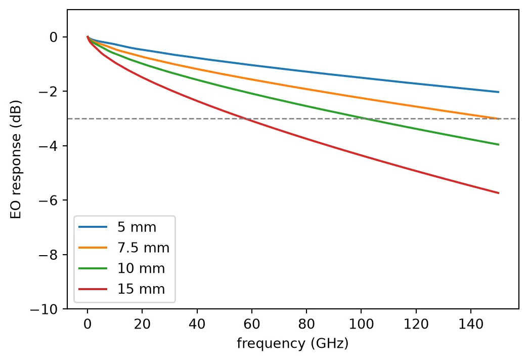

The transmitter uses a 10 mm modulator. Its half-wave voltage is under 3 V, which a driver amplifier for 120 GBd delivers, and its EO bandwidth is near 100 GHz, beyond the 66 GHz the signal occupies. A 15 mm line would halve the drive power but fall to about 60 GHz. The link page filters the drive voltage with this response, so the modulator bandwidth enters the link simulation through the extracted line, not through a single pole.

Time-domain model of the modulator

The MZM of the PDK is a circuit of two MMIs and two phase-shifter arms. Its arms have no drive ports in that circuit, because the T-rail line is a separate electrical waveguide. PhotonForge has a stepper for a travelling-wave arm, TerminatedModTimeStepper. It holds the same line as the response above: impedance, microwave index, frequency-dependent loss, load and optical group index. A push-pull MZM needs two such arms that get the same voltage with opposite signs. The PDK cell has no place for that inverted drive.

The link therefore uses a different form that gives the same field:

• The phase is linear in the voltage. The Pockels effect changes the index in proportion to the field. Each arm’s phase is therefore the drive voltage, filtered by the response of the line.
• The filter can move to the drive. A linear filter on the voltage gives the same phase whether the electrode applies it or the drive signal carries it. The MZM transfer, a sine of the phase difference, then acts on that phase.
• The response is not a single pole. The RF loss grows with $\sqrt{f}$, the microwave and optical waves walk off, and the load reflects. The f_3dB of the MZM stepper is one pole, so it stays at zero.

The cell below makes the model of the MZM: a TwoPortModel whose time stepper is MZMTimeStepper. The stepper has the half-wave voltage of the 10 mm line and the loss of the arms and the two MMIs. Its bias point is the null, as QAM needs. Its v_pi is the voltage that shifts one arm by $\pi$, so push-pull reaches $\pi$ between the arms at half of it. The cell sets every parameter of the stepper, including the ones this link leaves at zero. The chip layout gives this model to each MZM when it places the MZM.

modulation_length = 10000.0  # Length of the T-rail electrode of the chip (um)
arm_loss = 0.2  # Optical loss of each arm over 1 cm (dB)

# Excess loss of one MMI at the design wavelength, from the FDTD result
mmi_excess = -10 * np.log10(np.interp(lda0, wls, t1 + t2))

# Model of the MZM: its S matrix holds only a constant transmission, and the link uses its stepper
modulator_model = pf.TwoPortModel(t=0.5)
# Time stepper of the MZM; the drive voltage carries the response of the line
modulator_model.time_stepper = pf.MZMTimeStepper(
    v_pi=2 * vpil_eff / modulation_length,  # Voltage that shifts one arm by pi (V)
    z0=50.0,  # Impedance of the drive port (ohm)
    extinction_ratio=None,  # Extinction ratio: infinite, the two arms are balanced
    insertion_loss=arm_loss + 2 * mmi_excess,  # Loss of the arms and the two MMIs (dB)
    f_3dB=0,  # Bandwidth of the stepper: none, the drive carries it
    phase_bias=180.0,  # Phase difference between the arms at zero drive (degrees)
    k2=0.0,  # Quadratic electro-optic coefficient: none, the Pockels effect is linear (rad/V^2)
    k3=0.0,  # Cubic electro-optic coefficient (rad/V^3)
    dloss_dv=0.0,  # Change of the loss with the drive: none in lithium niobate (dB/V)
    dloss_dv2=0.0,  # Quadratic change of the loss with the drive (dB/V^2)
)
print(f"V_pi {vpil_eff / modulation_length:.2f} V push-pull, insertion loss {arm_loss + 2 * mmi_excess:.2f} dB")

V_pi 2.95 V push-pull, insertion loss 0.39 dB

Bias heater

Each MZM is biased at its null, where the field passes through zero and changes sign, and the nested interferometer sets 90 degrees between I and Q. These operating points drift with temperature and with the slow charge relaxation of lithium niobate, so they are held by heaters. The PDK’s heated_straight is a 1 um gold strip 0.9 um thick, 1 um above the film and 1.22 um to the side of a 1 um ridge, 700 um long.

The power for a $\pi$ shift follows from a 2D heat simulation of the cross-section and a mode solve of the heated waveguide. The structures of the heat simulation come from the PDK cell itself: Component.extrude with classification="electrical" returns the solids of the drawn layout with the electrical half of each material, so the geometry is exactly what the PDK draws. The PDK’s electrical media describe the microwave behaviour only, so the cell below builds the technology again with a thermal conductivity, a heat capacity and a density added to each of them, through the technology’s own material arguments. The gold keeps its microwave model, which the PDK’s transmission-line ports rely on, and gains a heat specification on top of it.

The heater is uniform along its 700 um, so a cross-section halfway along it is a 2D problem. Each extruded solid is cut at that plane and extended along the waveguide, which is the form a 2D heat simulation needs. The simulation puts 0.1 mW per micrometre into the heater and holds the bottom of the silicon handle at room temperature. The heater sits 1.22 um to the side of the ridge, so it does not absorb the light, and the hottest part of the film is beside the ridge rather than in it.

The temperature rise then raises the extraordinary index of lithium niobate by $3.34 \times 10^{-5}$ per kelvin [5], and the oxide by $0.95 \times 10^{-5}$ per kelvin. Since both steps are linear, one power level is enough.

p_per_um = 1e-4  # Heater power per unit length (W/um), 0.1 mW/um
k = lambda w_per_m_k: w_per_m_k * 1e-6  # W/(m K) to W/(um K)

# Thermal properties: conductivity W/(m K), heat capacity J/(kg K), density kg/um^3
def with_heat(media, name, conductivity, capacity, density):
    heat = td.SolidSpec(conductivity=k(conductivity), capacity=capacity, density=density)
    return {"optical": media["optical"], "electrical": media["electrical"].updated_copy(heat_spec=heat, name=name)}

# The PDK technology again, with heat properties on its own electrical media
pdk = tech.parametric_kwargs
tech_heat = lx.lnoi400(
    ln=with_heat(pdk["ln"], "LN", 4.6, 628, 4.64e-15),
    sio2=with_heat(pdk["sio2"], "SiO2", 1.38, 740, 2.2e-15),
    si=with_heat(pdk["si"], "Si", 148, 711, 2.33e-15),
    metal=with_heat(pdk["metal"], "Au", 317, 129, 19.3e-15),
)

# The PDK heater cell, extruded as drawn. A drawing-only rectangle widens the cell to 200 um, so the
# blanket layers (handle wafer, oxide, slab) extend as far as the simulation domain.
heater_cell = lxc.heated_straight(technology=tech_heat)
heater_length = heater_cell.ports["P1"].center[0] - heater_cell.ports["P0"].center[0]
x_cut = heater_length / 2  # The cross-section is taken halfway along the heater
heater_cut = pf.Component("HEATER_CUT", technology=tech_heat)
heater_cut.add_reference(heater_cell)
heater_cut.add("DOC", pf.Rectangle((x_cut - 10, -100), (x_cut + 10, 100)))
structures = [solid.to_tidy3d() for solid in heater_cut.extrude(classification="electrical")]
# Heater cross-section from the PDK parameters, and the domain: 100 um of handle wafer below the oxide
heater_width = 1.0  # heated_straight default (um)
heater_thickness = pdk["tl_thickness"]
z_top = pdk["ln_thickness"] + pdk["tl_separation"] + heater_thickness  # top of the gold
z_bottom = -pdk["box_thickness"] - 100.0
# the domain, in the (y, z) plane
window = shapely.geometry.box(-100, z_bottom, 100, z_top)

# A 2D heat solve needs structures that are uniform along x: cut each extruded solid at x_cut,
# keep the part inside the domain (the handle wafer reaches -Z_INF) and extend it along x.
# The heat solver takes each medium's thermal part; the gold is the source, so it gets a name.
cross_section = []
for s in structures:
    shapes = [shapely.intersection(p, window) for p in s.geometry.intersections_plane(x=x_cut)]
    slabs = [
        td.PolySlab(vertices=list(p.exterior.coords)[:-1], axis=0, slab_bounds=(-td.inf, td.inf))
        for p in shapes
        if not p.is_empty
    ]
    cross_section.append(
        td.Structure(
            geometry=td.GeometryGroup(geometries=slabs),
            medium=td.MultiPhysicsMedium(heat=s.medium.heat_spec, name=s.medium.name),
            name="heater" if s.medium.name == "Au" else None,
        )
    )

heat_sim = td.HeatChargeSimulation(
    center=(x_cut, 0, (z_bottom + z_top) / 2),
    size=(0, 200, z_top - z_bottom),
    structures=cross_section,
    medium=td.MultiPhysicsMedium(heat=tech_heat.parametric_kwargs["sio2"]["electrical"].heat_spec, name="SiO2"),
    # Volume heat rate (W/um^3) that gives p_per_um in the heater cross-section
    sources=[td.HeatSource(structures=["heater"], rate=p_per_um / (heater_width * heater_thickness))],
    boundary_spec=[
        td.HeatChargeBoundarySpec(
            condition=td.TemperatureBC(temperature=300),
            placement=td.SimulationBoundary(surfaces=["z-"]),
        ),
        td.HeatChargeBoundarySpec(
            condition=td.HeatFluxBC(flux=0),
            placement=td.SimulationBoundary(surfaces=["z+", "y-", "y+"]),
        ),
    ],
    # The monitor covers the waveguide and the heater above it
    monitors=[
        td.TemperatureMonitor(
            center=(x_cut, 0, (z_top - 1.0) / 2), size=(0, 6.0, z_top + 1.0), name="T", unstructured=True
        )
    ],
    grid_spec=td.DistanceUnstructuredGrid(
        dl_interface=0.02,
        dl_bulk=3.0,
        distance_interface=0.05,
        distance_bulk=8.0,
        relative_min_dl=0,
        sampling=200,
        mesh_refinements=[
            td.GridRefinementRegion(
                center=(x_cut, 0, 0.4), size=(0, 8.0, 3.0), dl_internal=0.03, transition_thickness=1.0
            )
        ],
    ),
)
heat_data = web.run(heat_sim, task_name="heater_heat_pdk_layout", verbose=False)
temperature = heat_data["T"].temperature

# Temperature rise on a regular grid around the waveguide, for the perturbed mode solve
ys, zs = np.linspace(-3, 3, 121), np.linspace(-0.6, 1.6, 89)
d_temp = np.nan_to_num(temperature.interp(x=x_cut, y=ys, z=zs, fill_value=300.0).values[0] - 300.0)
print(f"temperature rise at the waveguide up to {d_temp.max():.1f} K at {p_per_um * 1e3:.1f} mW/um")

# The whole monitor, with the outline of every structure drawn on top
z_plot = np.linspace(-1.0, z_top, 140)
t_plot = np.nan_to_num(temperature.interp(x=x_cut, y=ys, z=z_plot, fill_value=300.0).values[0] - 300.0)
fig, ax = plt.subplots(1, 1, figsize=(8, 4.2))
im = ax.pcolormesh(ys, z_plot, t_plot.T, shading="auto", cmap="inferno")
fig.colorbar(im, ax=ax, label="temperature rise (K)")
for s in cross_section:
    s.geometry.plot(x=x_cut, ax=ax, facecolor="none", edgecolor="w", linewidth=1)
ax.set_xlim(-3, 3)
ax.set_ylim(-1.0, z_top)
ax.set_aspect("equal")
ax.set_xlabel("y (um)")
ax.set_ylabel("z (um)")
ax.set_title(f"temperature rise at {p_per_um * 1e3:.1f} mW/um")
plt.show()

temperature rise at the waveguide up to 53.3 K at 0.1 mW/um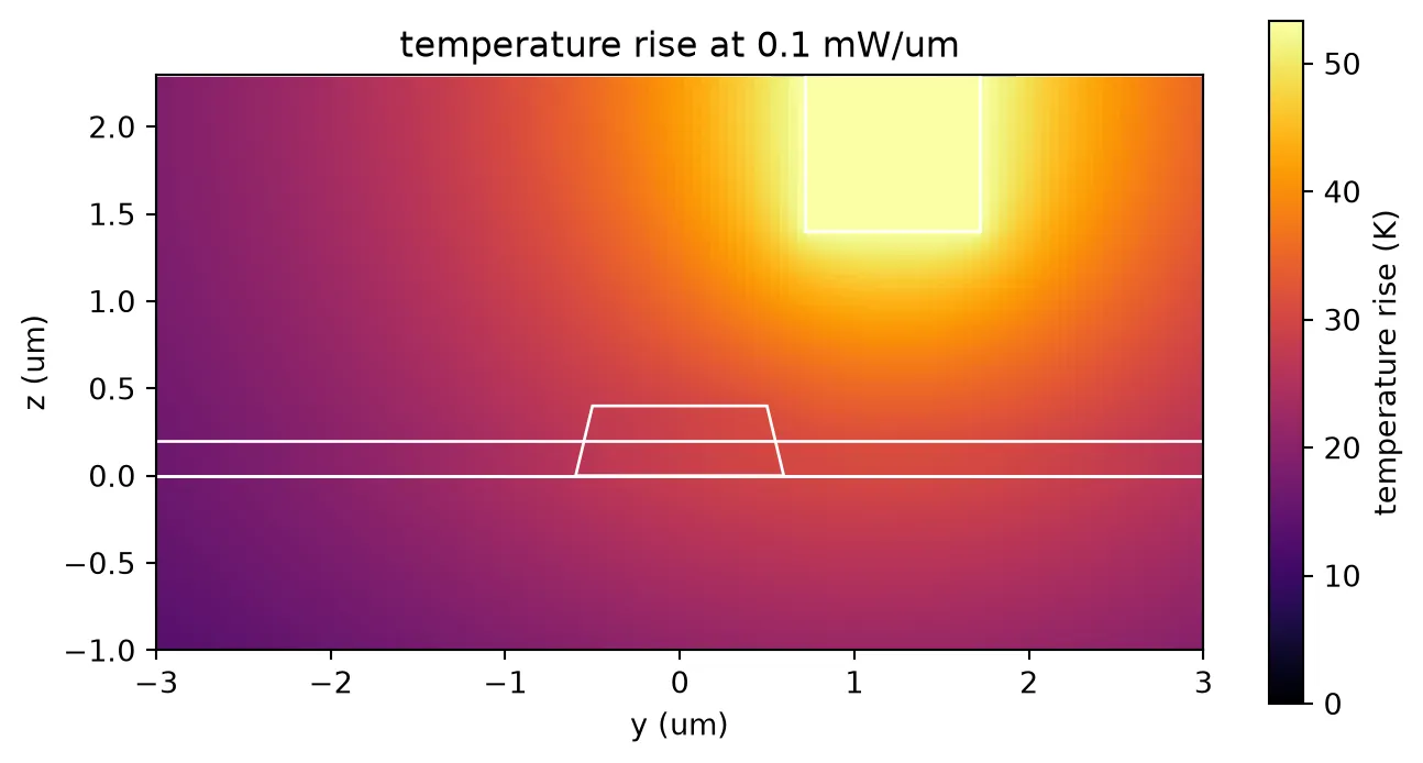

# Indices at room temperature, from the PDK materials
ln_pdk = tech.parametric_kwargs["ln"]
n_o = float(np.sqrt(ln_pdk["optical"].xx.eps_model(f0).real))
n_e_pdk = float(np.sqrt(ln_pdk["optical"].yy.eps_model(f0).real))
ox_pdk = tech.parametric_kwargs["sio2"]
n_ox = float(np.sqrt(ox_pdk["optical"].eps_model(f0).real))

# The PDK waveguide, solved cold and with the temperature map written into the indices
w_wg = 1.0  # Ridge width of the PDK waveguide (um)
heater_arm = pf.PortSpec(
    "arm",
    width=6.0,
    limits=(-1.5, 1.6),
    num_modes=1,
    target_neff=2.0,
    path_profiles=((w_wg, 0, (2, 0)), (12.0, 0, (3, 0))),
)
coords = {"x": [0.0], "y": ys, "z": zs}
one = td.SpatialDataArray(np.ones((1, 1, 1)), coords={"x": [0], "y": [0], "z": [0]})
n_eff_heat = []
for scale in (0.0, 1.0):
    dt = td.SpatialDataArray(scale * d_temp[None, :, :], coords=coords)
    ln_hot = td.CustomAnisotropicMedium(
        xx=td.CustomMedium(permittivity=n_o**2 * one, subpixel=True),
        yy=td.CustomMedium(permittivity=(n_e_pdk + 3.34e-5 * dt) ** 2, subpixel=True),
        zz=td.CustomMedium(permittivity=n_o**2 * one, subpixel=True),
    )
    ox_hot = td.CustomMedium(permittivity=(n_ox + 0.95e-5 * dt) ** 2, subpixel=True)
    tech_hot = lx.lnoi400(
        ln={"optical": ln_hot, "electrical": ln_pdk["electrical"]},
        sio2={"optical": ox_hot, "electrical": ox_pdk["electrical"]},
    )
    # The slanted sidewalls need subpixel averaging, which port_modes provides
    ms = pf.port_modes(
        heater_arm, [f0], mesh_refinement=30, technology=tech_hot, verbose=False, show_progress=False
    )
    n_eff_heat.append(float(np.real(ms.data.n_eff.values.ravel()[0])))

# A pi shift needs dn_eff L = lambda / 2; the index change scales with the power per length
dn_heat = n_eff_heat[1] - n_eff_heat[0]
p_pi = lda0 / 2 / (heater_length * dn_heat) * p_per_um * heater_length
print(f"dn_eff {dn_heat:.2e} at {p_per_um * 1e3:.1f} mW/um")
print(f"P_pi {p_pi * 1e3:.0f} mW for the {heater_length:.0f} um heater")

dn_eff 8.52e-04 at 0.1 mW/um
P_pi 91 mW for the 700 um heater

A $\pi$ shift costs about 90 mW. The bias of an MZM at its null and the 90 degree offset of each IQ modulator need at most half of that once the chip is characterized, so six heaters stay within a few hundred milliwatts. The heaters set operating points only, so the link simulation treats the biases as set and does not need a heater model.

Polarization rotator-combiner

The PRC takes the two TE outputs of the IQ modulators and sends them into one waveguide, one as TE0 and the other as TM0. It is an adiabatic mode-evolution device after Gan et al. [4]: a narrow ridge runs beside the 1 um ridge, starts at 250 nm and widens to 650 nm over 1.5 mm, and the gap between them then opens. Light launched in TM0 of the wide ridge evolves into TE1 where TM0 and TE1 have the same index, which the slanted sidewalls make possible, and TE1 of the pair becomes TE0 of the narrow ridge as the ridges separate. TE0 of the wide ridge stays where it is. Used backwards, the device combines: TE0 into the narrow arm comes out as TM0, and TE0 into the wide arm comes out as TE0.

The cell below draws the device with the PDK layers. The narrow tip is the 250 nm minimum ridge width of the design rules.

@pf.parametric_component(name_prefix="PRC")
def prc(
    *,
    w0=1.0,  # Wide ridge (um)
    # Narrow ridge at its tip: the minimum ridge width of the design rules
    w1_start=0.25,
    w1_end=0.65,  # Narrow ridge at the end of the evolution section
    gap_far=1.4,  # Gap where the ridges do not interact
    gap=0.4,  # Gap in the evolution section
    lead=10.0,
    length_in=100.0,
    length_evolution=1500.0,
    length_out=140.0,
    length_widen=50.0,
    bend_length=100.0,
    bend_offset=10.0,
    model=None,
):
    c = pf.Component()
    ridge, slab = "LN_RIDGE", "LN_SLAB"
    x0 = lead
    x1 = x0 + length_in
    x2 = x1 + length_evolution
    x3 = x2 + length_out
    x4 = x3 + length_widen

    # The wide ridge runs straight through
    c.add(ridge, pf.Rectangle((0, -w0 / 2), (x4, w0 / 2)))

    # Narrow ridge: constant tip, linear width taper, gap opens, then widens to w0 for the output
    xs = [x0, x1, x2, x3, x4]
    gaps = [gap_far, gap, gap, gap_far, gap_far]
    widths = [w1_start, w1_start, w1_end, w1_end, w0]
    inner = [(x, -(w0 / 2 + g)) for x, g in zip(xs, gaps)]
    outer = [(x, -(w0 / 2 + g + w)) for x, g, w in zip(xs, gaps, widths)]
    c.add(ridge, pf.Polygon(inner + outer[::-1]))

    # The PDK S-bend takes the rotated arm away; a straight of the same length keeps P1 aligned
    bend = lxc.s_bend_spline(length=bend_length, offset=-bend_offset)
    narrow_end = (x4, -(w0 / 2 + gap_far + w0 / 2))
    r_bend = c.add_reference(bend)
    r_bend.connect("P0", pf.Port(narrow_end, 180, "RWG1000"))
    x_end = r_bend["P1"].center[0]
    p2 = r_bend["P1"]
    c.add(ridge, pf.Rectangle((x4, -w0 / 2), (x_end, w0 / 2)))

    # The S-bend's shapes are copied into the cell rather than referenced, so the rotator-combiner
    # is one device with three ports, as the layout check treats it
    for layer in (ridge, slab):
        shapes = r_bend.get_structures(pf.config.default_technology.layers[layer].layer)
        if shapes:
            c.add(layer, *shapes)
    c.remove(r_bend)

    # Slab drawn as keep-LN around everything, as the PDK cells do
    c.add(slab, pf.envelope(c, offset=4.5))

    # P0 carries TE0 and TM0; P1 and P2 are the single-mode TE arms
    two_mode = pf.config.default_technology.ports["RWG1000"].copy()
    two_mode.num_modes = 2
    c.add_port(pf.Port((0, 0), 0, two_mode), "P0")
    c.add_port(pf.Port((x_end, 0), 180, "RWG1000"), "P1")
    c.add_port(p2, "P2")
    if model is not None:
        c.add_model(model, "EME data")
    return c

viewer(prc())

The device is 1.9 mm long and 1 um wide in most places, which makes FDTD expensive and eigenmode expansion (EME) the natural solver: EME propagates the modes of each cross-section through the slowly varying structure. The coefficients were computed with an EMEModel at 1500, 1550 and 1600 nm, on a cell grid refined in the evolution section, and the group delay of each path from the local group indices along the device. Both are loaded from data files below and turned into a PolarizationSplitterRotatorModel. Each path is the EME amplitude times its own delay. The model samples them on a dense frequency grid because a 14 ps path delay turns the phase quickly with frequency.

rows = json.load(open("misc/coherent_prc_coefficients.json"))
delay = json.load(open("misc/coherent_prc_delay.json"))
wl_eme = np.array([row["wl"] for row in rows])
f_eme = pf.C_0 / wl_eme
coefficient = lambda key: np.array([complex(*row[key]) for row in rows])

# Group delay of each route: the device up to x = 1800 um, then the output arm, which is a 100 um
# straight for TE and the longer S-bend for TM
core_te = np.trapezoid(delay["ng_te"], delay["xs"])
core_tm = np.trapezoid(delay["ng_tm"], delay["xs"])
tail = 100.0 * delay["ng_out"]
tau = {
    "TE": (core_te + tail) / pf.C_0,
    "TM": (core_tm + tail + delay["extra_bend_um"]) / pf.C_0,
}
print(f"X/Y skew {(tau['TM'] - tau['TE']) * 1e12:.3f} ps")

# Magnitude from EME, phase from the 1550 nm EME value plus the route's delay
i0 = int(np.argmin(abs(wl_eme - lda0)))
f_model = pf.C_0 / np.linspace(1.45, 1.65, 6001)

def path(key, route):
    mag = np.interp(f_model, f_eme[::-1], np.abs(coefficient(key))[::-1])
    phase = np.angle(coefficient(key)[i0]) + 2 * np.pi * (f_model - f_eme[i0]) * tau[route]
    return pf.Interpolator(f_model, mag * np.exp(1j * phase), coords="mag_phase")

prc_model = pf.PolarizationSplitterRotatorModel(
    s02=path("TE->TE_thr", "TE"),  # P0 TE0 to P1, the wide arm
    s04=path("TE->TE_cro", "TE"),  # P0 TE0 to P2, leakage
    s12=path("TM->TE_thr", "TE"),  # P0 TM0 to P1, leakage
    s14=path("TM->TE_cro", "TM"),  # P0 TM0 to P2, the rotated arm
    output_mode=0,
)
prc_cell = prc(model=prc_model)

# The combiner direction: X into the wide arm, Y into the rotated arm
wl_plot = np.linspace(1.50, 1.60, 101)
s_prc = prc_cell.s_matrix(pf.C_0 / wl_plot)
db = lambda a, b: 20 * np.log10(np.abs(s_prc[(a, b)]))
fig, ax = plt.subplots(1, 1, figsize=(6, 4))
ax.plot(wl_plot * 1e3, db("P1@0", "P0@0"), label="X: P1 to TE0")
ax.plot(wl_plot * 1e3, db("P2@0", "P0@1"), label="Y: P2 to TM0")
ax.plot(wl_plot * 1e3, db("P1@0", "P0@1"), "--", label="X leaking into TM0")
ax.plot(wl_plot * 1e3, db("P2@0", "P0@0"), "--", label="Y leaking into TE0")
ax.set_xlabel("wavelength (nm)")
ax.set_ylabel("transmission (dB)")
ax.legend()
plt.show()
for label, key in (("X", ("P1@0", "P0@0")), ("Y", ("P2@0", "P0@1"))):
    print(f"{label} loss at 1550 nm {-np.interp(lda0, wl_plot, db(*key)):.3f} dB")
print(f"largest leakage into the other polarization {max(db('P1@0', 'P0@1').max(), db('P2@0', 'P0@0').max()):.1f} dB")

X/Y skew 0.197 ps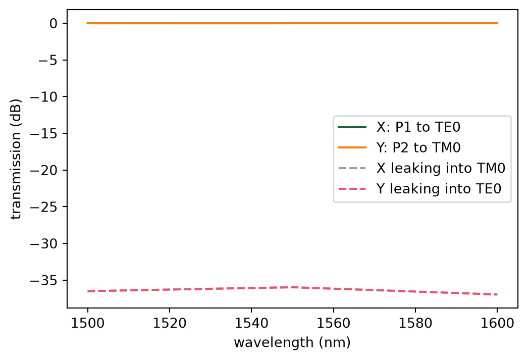

X loss at 1550 nm 0.001 dB
Y loss at 1550 nm 0.004 dB
largest leakage into the other polarization -36.0 dB

Both polarizations pass with a loss of a few thousandths of a decibel, because the mode evolution is adiabatic over the whole band, and each leaks below $-35$ dB into the other. The two routes differ in length by a fraction of a picosecond, which the receiver equalizer absorbs. The link page uses this model.

Gan et al. [4] report an insertion loss below 0.13 dB and an extinction ratio above 18 dB over 230 nm in simulation, and below 0.5 dB and above 20 dB over 110 nm in measurement. The same EME setup, applied to their stack with sidewalls 30 degrees from vertical, places the TM0-TE1 anticrossing at the same narrow-ridge width as their paper, 0.36 um. On LNOI400 the device performs better for three reasons:

• A longer evolution section. The steeper sidewalls of LNOI400, 13.5 degrees from vertical, move the anticrossing to a 0.42 um narrow ridge and make it narrower, with a minimum index splitting of 0.0078 instead of 0.0095. The evolution section is therefore 1.5 mm long instead of 1 mm, and a slower evolution is a more adiabatic one: less power is left in the wrong supermode, which is where both the loss and the leakage come from.
• A tip at the design-rule minimum. The narrow ridge starts at 250 nm, far from the anticrossing, so the input supermodes are almost pure TE0 and TM0 of the wide ridge.
• What EME leaves out. EME propagates the modes of an ideal structure. Sidewall roughness, material absorption and fabrication errors in the ridge widths are not in the model, and they account for most of the difference between Gan’s simulated and measured loss. A fabricated device on LNOI400 would sit closer to their measured 0.5 dB than to the thousandths of a decibel computed here.

The two cells below recompute the data files, commented out because the EME run takes about an hour per wavelength. The first runs an EMEModel on the drawn device, with 20 cells in the input section, 150 in the evolution section and 28 after it, and writes the four through and leakage coefficients. The second solves the cross-section of the two ridges along the device and integrates the group index of each route, which gives the delays.

# # EME of the drawn device: one subgrid per section, 8 modes per cell
# mode_spec = td.EMEModeSpec(num_modes=8)
# x_in, x_evo = 10.0 + 100.0, 10.0 + 100.0 + 1500.0  # ends of the input and evolution sections
# eme_grid = td.EMECompositeGrid(
#     subgrids=[td.EMEUniformGrid(num_cells=n, mode_spec=mode_spec) for n in (20, 150, 28)],
#     subgrid_boundaries=[x_in, x_evo],
# )
# prc_eme = prc(model=pf.EMEModel(eme_grid_spec=eme_grid, grid_spec=40, verbose=False))
# wl_run = [1.50, 1.55, 1.60]
# s_eme = prc_eme.s_matrix([pf.C_0 / wl for wl in wl_run])
# pair = lambda a, b: [[float(np.real(v)), float(np.imag(v))] for v in s_eme[(a, b)]]
# zero = [[0.0, 0.0]] * len(wl_run)  # P1 and P2 are single-mode TE, so no TM output
# rows = [
#     {"wl": wl, "TE->TE_thr": pair("P0@0", "P1@0")[k], "TE->TE_cro": pair("P0@0", "P2@0")[k],
#      "TM->TE_thr": pair("P0@1", "P1@0")[k], "TM->TE_cro": pair("P0@1", "P2@0")[k],
#      "TE->TM_thr": zero[k], "TE->TM_cro": zero[k], "TM->TM_thr": zero[k], "TM->TM_cro": zero[k]}
#     for k, wl in enumerate(wl_run)
# ]
# with open("misc/coherent_prc_coefficients.json", "w") as file:
#     json.dump(rows, file)

# # Group index of the two lowest supermodes of the ridge pair, sampled along the device
# def pair_spec(w1, g):
#     return pf.PortSpec("two ridges", width=8, limits=(-1.5, 1.9), num_modes=4, target_neff=2.2,
#                        path_profiles=[(1.0, g / 2 + 0.5, (2, 0)), (w1, -(g / 2 + w1 / 2), (2, 0)), (12, 0, (3, 0))])
# samples = (
#     [(10 + 100 * t, 0.25, 1.4 - 1.0 * t) for t in np.linspace(0, 1, 4)]
#     + [(110 + 1500 * t, 0.25 + 0.4 * t, 0.4) for t in np.linspace(0, 1, 13)[1:]]
#     + [(1610 + 140 * t, 0.65, 0.4 + 1.0 * t) for t in np.linspace(0, 1, 4)[1:]]
#     + [(1750 + 50 * t, 0.65 + 0.35 * t, 1.4) for t in np.linspace(0, 1, 3)[1:]]
# )
# xs, ng_te, ng_tm = [0.0], [], []
# for x, w1, g in samples:
#     d = pair_spec(w1, g).to_tidy3d([f0], mesh_refinement=40, group_index=True, technology=tech).solve()
#     xs.append(x)
#     ng_te.append(float(d.n_group.isel(f=0).values[0]))  # TE0 of the wide ridge
#     ng_tm.append(float(d.n_group.isel(f=0).values[1]))  # the mode TM0 evolves along
# ng_te, ng_tm = [ng_te[0]] + ng_te, [ng_tm[0]] + ng_tm
# ng_out = float(pf.port_modes("RWG1000", [f0], group_index=True).data.n_group.values.ravel()[0])
# # The rotated arm leaves through an S-bend, longer than the straight beside it
# bend_extra = (pf.route_length(lxc.s_bend_spline(length=100.0, offset=-10.0)) - 100.0) * ng_out
# with open("misc/coherent_prc_delay.json", "w") as file:
#     json.dump(dict(xs=xs, ng_te=ng_te, ng_tm=ng_tm, ng_out=ng_out, extra_bend_um=bend_extra), file)

Edge coupler

The PDK edge coupler is a bilayer taper: the ridge narrows to a tip while the slab underneath narrows more slowly, so the mode expands into a large, weakly guided spot at the facet. It is designed for a 3 um mode field diameter, as delivered by a lensed fiber. The coupler is long compared with the facet region, so it was simulated in two 3D FDTD parts: the facet and the first 40 um of taper, with a Gaussian beam launched in front of the facet, and the remaining taper to the 1 um ridge, launched in the fundamental mode at the 40 um cut. The product of the two transmissions is the coupler loss, for TE and for TM. Each part has one mirror symmetry plane, which also selects the polarization.

The fiber is modelled as a GaussianPort: a Gaussian beam with a 3 um mode field diameter, launched in air 3 um in front of the facet with its waist on the facet. This is what a lensed fiber delivers, and it is the fiber the PDK coupler is designed for: the lens forms a small spot in free space, at a working distance from the chip. A FiberPort describes something else, the guided mode of a cleaved fiber whose glass touches the facet, as the receiver page uses for a high numerical aperture fiber. With a 3.2 um fiber mode instead of the 3 um beam, the overlap would change by less than 0.02 dB, but the glass would replace the air in front of the facet and remove the reflection at the air to oxide interface, about 3 % or 0.15 dB. A FiberPort would therefore predict a slightly lower loss for a package this coupler is not designed for.

ec = lxc.edge_coupler()
viewer(ec)

ec_data = json.load(open("misc/coherent_tx_edge_coupler.json"))
fig, ax = plt.subplots(1, 1, figsize=(6, 4))
for pol in ("TE", "TM"):
    total_db = -10 * np.log10(np.array(ec_data[pol]["total"]))
    ax.plot(np.array(ec_data[pol]["wl"]) * 1e3, total_db, "o-", label=pol)
    print(f"{pol}: {np.interp(lda0, ec_data[pol]['wl'], total_db):.2f} dB at 1550 nm")
ax.set_xlabel("wavelength (nm)")
ax.set_ylabel("coupling loss (dB)")
ax.legend()
plt.show()

# The measured transmissions become the models of the coupler: the facet is P0, the waveguide P1.
# The FDTD gives power only, so the amplitude is its square root and the phase is zero.
f_ec = pf.C_0 / np.array(ec_data["TE"]["wl"])
t_te = np.sqrt(np.array(ec_data["TE"]["total"]))
t_tm = np.sqrt(np.interp(ec_data["TE"]["wl"], ec_data["TM"]["wl"], ec_data["TM"]["total"]))
ec.add_model(
    pf.DataModel(pf.SMatrix(f_ec, {("P0@0", "P1@0"): t_te, ("P1@0", "P0@0"): t_te}), interpolation_method="linear"),
    "FDTD data",
)
# The output coupler carries both polarizations: mode 0 is TE and mode 1 is TM at both ports
ec_two_mode_model = pf.DataModel(
    pf.SMatrix(
        f_ec,
        {("P0@0", "P1@0"): t_te, ("P1@0", "P0@0"): t_te, ("P0@1", "P1@1"): t_tm, ("P1@1", "P0@1"): t_tm},
    ),
    interpolation_method="linear",
)

TE: 0.91 dB at 1550 nm
TM: 1.75 dB at 1550 nm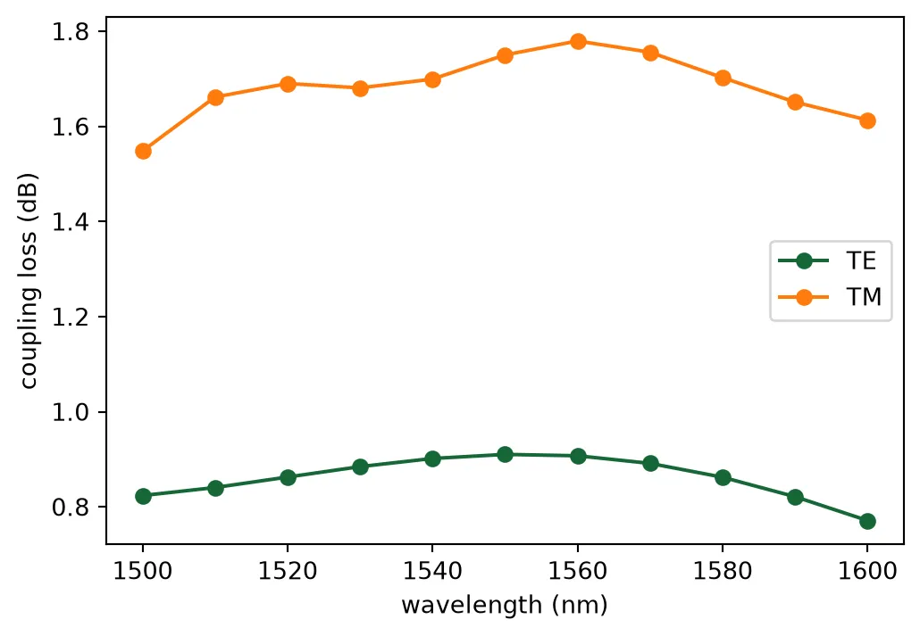

The cell below is the code that produced coherent_tx_edge_coupler.json, commented out because the four FDTD runs take about 10 FlexCredits together.

# # Air in front of the facet, on a layer of its own
# tech_ec = lx.lnoi400()
# tech_ec.add_layer("FACET_AIR", pf.LayerSpec((99, 1), "Air in front of the facet", "#ffffff18", "."))
# tech_ec.insert_extrusion_spec(
#     len(tech_ec.extrusion_specs),
#     pf.ExtrusionSpec(pf.MaskSpec((99, 1)), tech_ec.background_medium, (-pf.Z_INF, pf.Z_INF)),
# )
# ec_cell = lxc.edge_coupler(technology=tech_ec)
# x_cut, mfd, gap_fiber = 40.0, 3.0, 3.0  # cut position, fiber mode field diameter, fiber distance (um)
# w_cut = 0.25 + (2.05 - 0.25) * x_cut / 120.0  # lower-taper width at the cut, from the PDK defaults
# cut_spec = pf.PortSpec("cut", width=5.0, limits=tech_ec.ports["SWG250"].limits, num_modes=2,
#                        target_neff=1.6, path_profiles=[(w_cut, 0, (3, 0)), (12, 0, (3, 1))])
# out_spec = tech_ec.ports["RWG1000"].copy()
# out_spec.num_modes = 2
# wl_ec = np.linspace(1.50, 1.60, 11)
# result = {}
# for pol, sym in (("TE", -1), ("TM", 1)):
#     # Part 1: Gaussian beam, facet and taper up to the cut
#     facet = pf.Component(f"EC_FACET_{pol}", technology=tech_ec)
#     facet.add_reference(ec_cell)
#     facet.add("FACET_AIR", pf.Rectangle((-2 * gap_fiber, -12), (0, 12)))
#     facet.add_port(pf.GaussianPort(center=(-gap_fiber, 0, 0.1), input_vector=(1, 0, 0), waist_radius=mfd / 2,
#                                    waist_position=gap_fiber, polarization_angle=0 if pol == "TE" else 90), "G")
#     facet.add_port(pf.Port((x_cut, 0), 180, cut_spec), "C")
#     facet.add_model(pf.Tidy3DModel(grid_spec=12, symmetry=(0, sym, 0),
#                                    bounds=((None, -6.0, None), (x_cut + 2.0, 6.0, None)), verbose=False), "Tidy3D")
#     # Part 2: fundamental mode at the cut, through the rest of the taper to the output ridge
#     taper = pf.Component(f"EC_TAPER_{pol}", technology=tech_ec)
#     taper.add_reference(ec_cell)
#     taper.add_port(pf.Port((x_cut, 0), 0, cut_spec), "C")
#     taper.add_port(pf.Port(ec_cell.ports["P1"].center, ec_cell.ports["P1"].input_direction, out_spec), "P1")
#     taper.add_model(pf.Tidy3DModel(grid_spec=12, symmetry=(0, sym, 0),
#                                    bounds=((x_cut - 1.0, None, None), (None, None, None)), verbose=False), "Tidy3D")
#     t1 = np.abs(facet.s_matrix(pf.C_0 / wl_ec, model_kwargs={"inputs": ["G"]})[("G@0", "C@0")]) ** 2
#     t2 = np.abs(taper.s_matrix(pf.C_0 / wl_ec, model_kwargs={"inputs": ["C@0"]})[("C@0", "P1@0")]) ** 2
#     result[pol] = dict(wl=wl_ec.tolist(), facet=t1.tolist(), taper=t2.tolist(), total=(t1 * t2).tolist())
# with open("misc/coherent_tx_edge_coupler.json", "w") as file:
#     json.dump(result, file)

The transmitter only launches TE into its input coupler, but its output coupler carries both polarizations into the fiber, so the output sees the TE and TM losses together. Their difference is a polarization-dependent loss of the transmitter, which unbalances the two polarizations at the receiver. The link page includes it.

What comes next

The transmitter library is complete: the MMI, the 10 mm travelling-wave modulator, the heater, the PRC and the edge coupler, each with a measured response. The receiver page designs the receiver components, and the layout page draws both chips.