

Signal Integrity Analysis of a 100 Gbps Transmitter
High-speed optical modulators, operating at data rates of >100 Gbps per wavelength channel, requires careful attention to their time-domain response, since bandwidth limitations, dispersion, and non-ideal modulator transfer characteristics can degrade signal integrity and increase bit-error rates.
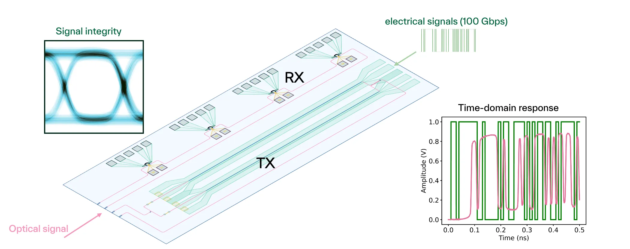
To evaluate quality of modulated signal in these systems, eye-diagram measurements are usually performed to visualize how the modulated signal evolves over time and reveal timing jitter, distortion, and noise margins.
Using PhotonForge, you can use scattering parameters to build a compact time-domain model of your component to analyze signal integrity, anticipate performance bottlenecks, and optimize design parameters before committing to costly fabrication.
import matplotlib.pyplot as pltimport numpy as npimport photonforge as pffrom scipy.signal import bessel, filtfiltHigh-speed modulator transfer function
Section titled “High-speed modulator transfer function”To begin, we create an electro-optic (EO) transfer function. In principle, one can also load experimentally measured EO S21 data as the transfer function.
For a traveling-wave EO modulator in thin-film lithium niobate, the frequency response (EO S21) follows the analytical expression [1]:
Here, is the angular microwave frequency,
is the transmission-line input impedance, and
account for forward/backward traveling waves. The propagation constant is , where is the microwave effective index, the (amplitude) loss rate in Np/m, the optical group index, the modulator length, the speed of light in vacuum, the load impedance, and the characteristic impedance.
Note: The source impedance is assumed equal to the load impedance.
References
- Zhu, Di, et al. “Integrated photonics on thin-film lithium niobate.” Advances in Optics and Photonics 13.2 (2021): 242–352, doi: 10.1364/AOP.411024.
def Mw(alpha_dB_per_cm_per_sqrtGHz, freq_GHz, n_m, n_g_opt, L_cm, Z_L, Z_0):    """    EO S21 of a traveling-wave modulator.
    Parameters    ----------    alpha_dB_per_cm_per_sqrtGHz : float        RF loss coefficient at 1 GHz scaling, in power dB/cm/√GHz.    freq_GHz : array_like        Microwave frequency in GHz.    n_m : float        Microwave effective index.    n_g_opt : float        Optical group index.    L_cm : float        Modulator length in cm.    Z_L, Z_0 : float        Load and characteristic impedances (ohms).
    Returns    -------    m_w : ndarray        EO S21.    """    L = L_cm * 1e-2    c = 299792458.0    omega = 2 * np.pi * (freq_GHz * 1e9)
    # dB/cm/√GHz -> Np/m at frequency f (GHz)    alpha_m = (        alpha_dB_per_cm_per_sqrtGHz * np.sqrt(freq_GHz) * (np.log(10) / 20.0) * 100.0    )
    gamma_m = alpha_m - 1j * (omega / c) * n_m
    F_plus = (1 - np.exp(gamma_m * L + 1j * (omega / c) * n_g_opt * L)) / (        gamma_m * L + 1j * (omega / c) * n_g_opt * L    )    F_minus = (1 - np.exp(-gamma_m * L + 1j * (omega / c) * n_g_opt * L)) / (        -gamma_m * L + 1j * (omega / c) * n_g_opt * L    )
    Z_in = Z_0 * (Z_L + Z_0 * np.tanh(gamma_m * L)) / (Z_0 + Z_L * np.tanh(gamma_m * L))
    m_w = (        (2 * Z_in / (Z_in + Z_L))        * ((Z_L + Z_0) * F_plus + (Z_L - Z_0) * F_minus)        / ((Z_L + Z_0) * np.exp(gamma_m * L) + (Z_L - Z_0) * np.exp(-gamma_m * L))    )
    return m_w
We can use our RF and optical solver to estimate these parameters like optical and RF indices, impedances, and also loss. Please refer to our notebook on designing electro-optic Mach-Zehnder Modulator.
# Initialize parameters with some nominal valuesfreq = np.logspace(-1, 2.5, 1001)  # GHz
alpha = 0.75  # dB/cm/sqrt(GHz) Transmission line loss in dB/cm/sqrt(GHz)n_m = 2.25  # microwave indexn_g_opt = 2.32  # optical group indexL_cm = 1  # modulator lengthZ_L = 50  # Assume 50 ohm termination loadZ_0 = 40  # Characteristic impedance of the tranmission line
# Electro-optic S21 calculated analytically# In reality this will be some measured data but this is good enough for nowEOS21 = Mw(alpha, freq, n_m, n_g_opt, L_cm, Z_L, Z_0)
fig, ax = plt.subplots(1, 2, figsize=(10, 3.5), tight_layout=True)
ax[0].plot(freq, 10 * np.log10(np.abs(EOS21) ** 2))ax[0].set(xlabel="Frequency (GHz)", ylabel="|EOS21| (dB)")
ax[1].plot(freq, np.angle(EOS21, deg=True))_ = ax[1].set(xlabel="Frequency (GHz)", ylabel="∠EOS21 (°)")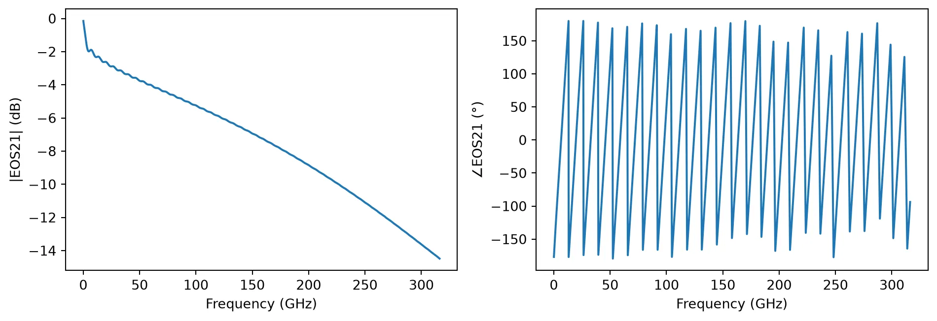
Building a time-domain model
Section titled “Building a time-domain model”Let’s first create a S-matrix representation in PhotonForge using the pole_residue_fit function.
baseband_freqs = freq * 1e9elements = {("1", "2"): EOS21}s_matrix = pf.SMatrix(frequencies=baseband_freqs, elements=elements)
# User vector fitting to fit the transfer function before building the time-domain modelpole_res, err = pf.pole_residue_fit(    s_matrix,    real=True,    min_poles=30,    max_poles=60,)s_fit = pole_res(baseband_freqs)
fig, ax = plt.subplots(1, 2, figsize=(10, 3.5), tight_layout=True)
ax[0].plot(freq, np.abs(EOS21))ax[0].plot(freq, np.abs(s_fit["1", "2"]), "--")ax[0].set(xlabel="Frequency (GHz)", ylabel="|EOS21|")
ax[1].plot(freq, np.angle(EOS21))ax[1].plot(freq, np.angle(s_fit["1", "2"]), "--")_ = ax[1].set(xlabel="Frequency (GHz)", ylabel="∠EOS21 (°)")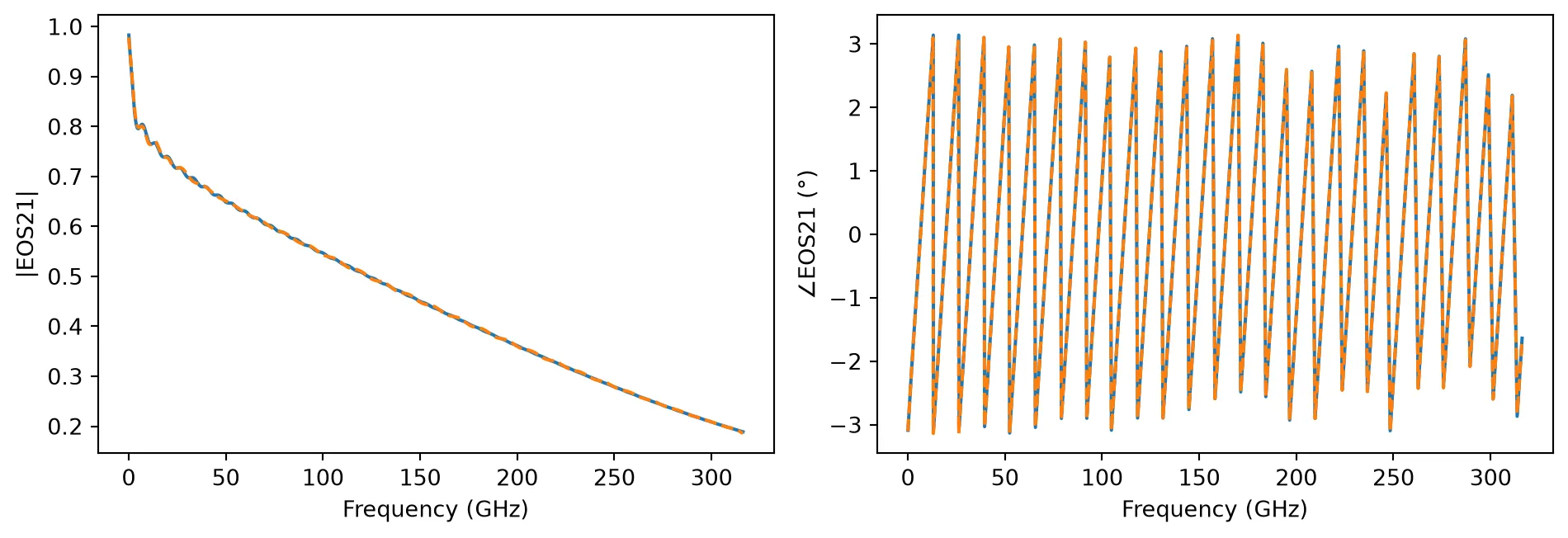
We see a warning about the RMS error tolerance for the fit. That is because the default tolerance is 1.0×10⁻⁴ (a very conservative value) and the fit reached 6×10⁻³. Nonetheless, we can see in the plot that all major features of the transfer function are captured, so we can move forward with this result.
PRBS Signal Generation
Section titled “PRBS Signal Generation”Next, we will generate the input electrical signal at 100 Gbps that would be applied to the modulator.
# Define parametersbit_rate = 100e9  # Bit rate (bps)T = 1 / bit_rate  # Bit period (s)num_bits = 1000  # Number of bits in PRBS sequenceV = 1  # peak driving voltage
# Desired samples per bit for smoother eye diagramsamples_per_bit = 100Fs = samples_per_bit * bit_rate  # Sampling frequencytime_step = 1 / Fs  # Time step for simulation
# Time vectort = np.arange(0, num_bits * T, time_step)
# Generate PRBS sequencenp.random.seed(0)  # For reproducibilityprbs_bits = np.random.randint(0, 2, num_bits)
# Generate NRZ signalideal_prbs_signal = np.repeat(prbs_bits, samples_per_bit)ideal_prbs_signal = V * ideal_prbs_signal[: len(t)]
fig, ax = plt.subplots(1, 1, figsize=(10, 3.5), tight_layout=True)ax.plot(t[:4000] * 1e12, ideal_prbs_signal[:4000])_ = ax.set(xlabel="Time (ps)", ylabel="Voltage (V)")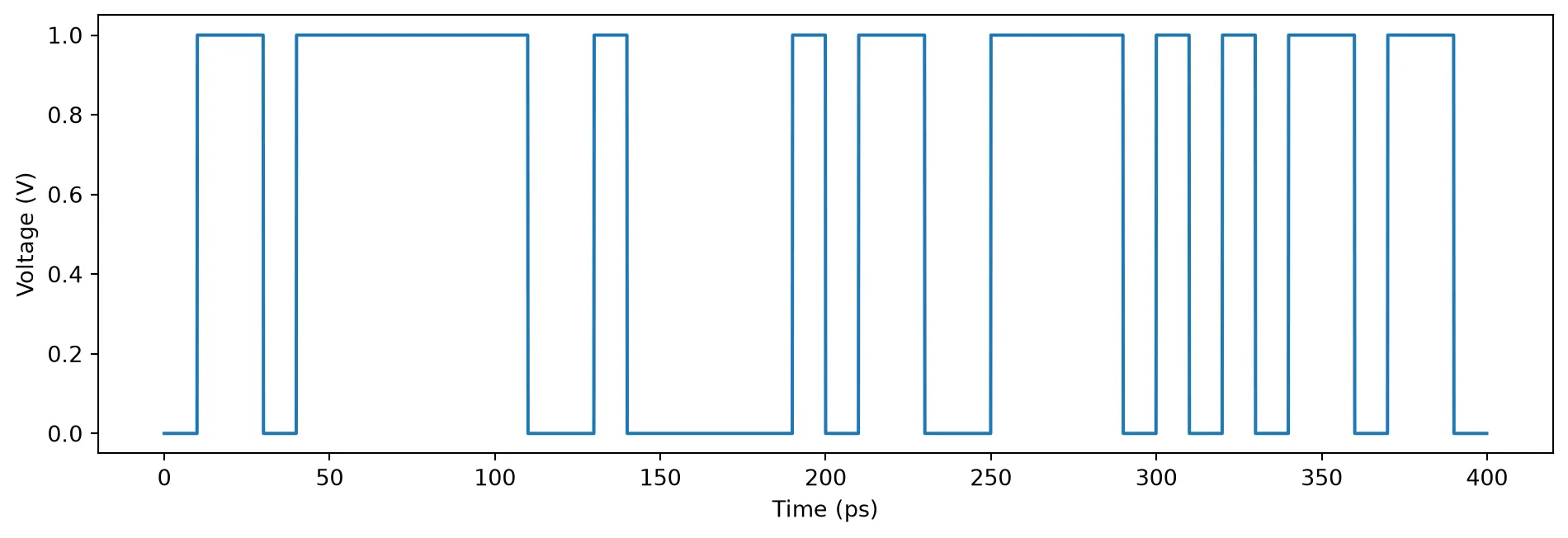
Real electrical systems have some high-frequency cutoff so the signals will not have sharp transitions like we generate above. In simulation, we must also guarantee that the major frequency components of the input signal fall within the valid region in our model, which was fitted up to 300 GHz.
Therefore, we’ll pipe the ideal signal through a 200 GHz low-pass-filter to generate the real electrical input.
cutoff_freq = 200e9  # 200 GHzfilter_order = 4
# Normalize the frequencynyquist_freq = 0.5 * Fsnormalized_cutoff = cutoff_freq / nyquist_freq
# Design Bessel filterb, a = bessel(N=filter_order, Wn=normalized_cutoff, btype="low", analog=False)
# Apply the filterreal_prbs_signal = filtfilt(b, a, ideal_prbs_signal)
fig, ax = plt.subplots(1, 1, figsize=(10, 3.5), tight_layout=True)ax.plot(t[:4000] * 1e12, ideal_prbs_signal[:4000], label="Ideal PRBS signal")ax.plot(t[:4000] * 1e12, real_prbs_signal[:4000], label="Real PRBS signal")ax.set(xlabel="Time (ps)", ylabel="Voltage (V)")_ = plt.legend()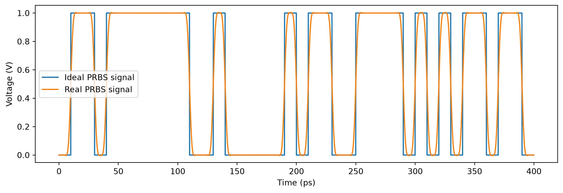
Build a time domain model
Section titled “Build a time domain model”First use the frequency response to build a time-domain model.
time_domain_model = pf.TimeDomainModel(pole_res, time_step)Now, time-step to generate output optical signal as a function of time
inputs = pf.TimeSeries(values={"1": real_prbs_signal}, time_step=time_step)optical_signal = np.abs(time_domain_model.step(inputs=inputs)["2"])fig, ax = plt.subplots(1, 1, figsize=(10, 3.5), tight_layout=True)ax.plot(t[:4000] * 1e12, real_prbs_signal[:4000], label="Input")ax.plot(t[:4000] * 1e12, optical_signal[:4000], label="Output")ax.set(xlabel="Time (ps)", ylabel="Amplitude")_ = plt.legend()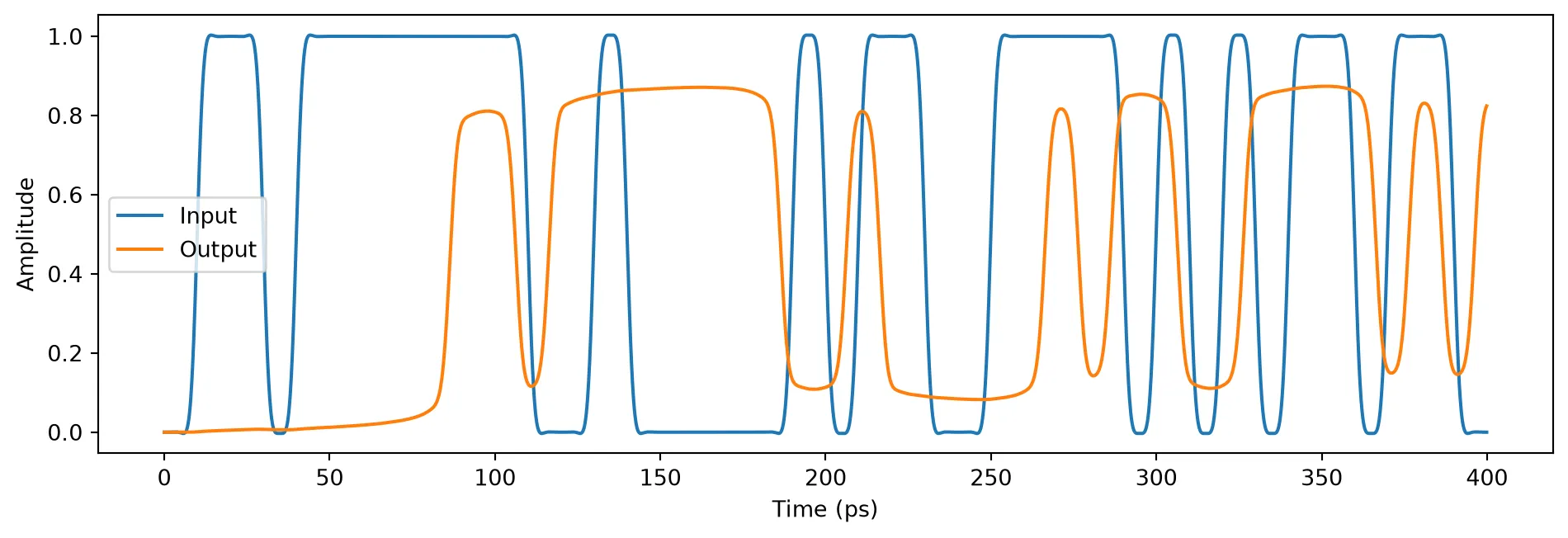
We can use the full sample extent to build an eye diagram.
def plot_eye_diagram(optical_output_signal, bit_rate, time_step):    Fs = 1 / time_step  # sampling frequency    samples_per_bit = int(0.5 + Fs / bit_rate)
    # Calculate window parameters    samples_per_window = 2 * samples_per_bit  # 2T window    start_index = samples_per_window  # Skip initial transients
    # Calculate number of windows    num_windows = (        len(optical_output_signal)        - start_index        - (samples_per_window - samples_per_bit)    ) // samples_per_bit    if num_windows <= 0:        raise ValueError("Output signal is too short to generate eye diagram.")
    # Extract signal segments for the eye diagram    parts = []    for k in range(num_windows):        idx_start = start_index + k * samples_per_bit        idx_end = idx_start + samples_per_window        part = optical_output_signal[idx_start:idx_end]        parts.append(part)
    parts = np.array(parts).T  # Transpose for time on x-axis
    # Time vector for plotting (centered around 0, in nanoseconds)    t = (np.arange(samples_per_window) - samples_per_bit) * time_step * 1e12
    # Plotting    fig, ax = plt.subplots(1, 1, figsize=(7, 4.5), tight_layout=True)    ax.plot(t, parts, color="yellow", alpha=0.1)    ax.set(xlabel="Time (ps)", ylabel="Amplitude", facecolor="k", xlim=(t[0], t[-1]))    ax.grid(ls=":")
plot_eye_diagram(optical_signal, bit_rate, time_step)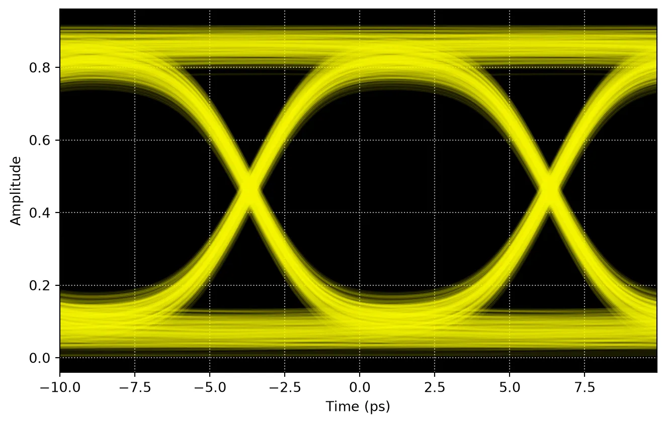
Since this modulator has relatively high bandwidth, it can support high speed modulation and you an see clear eye-opening for this 100 Gbps non-return-to-zero (NRZ) signal.