Fabrication-Aware Simulation: Two Coupled Ring Resonator Filter

Download notebook (.zip)

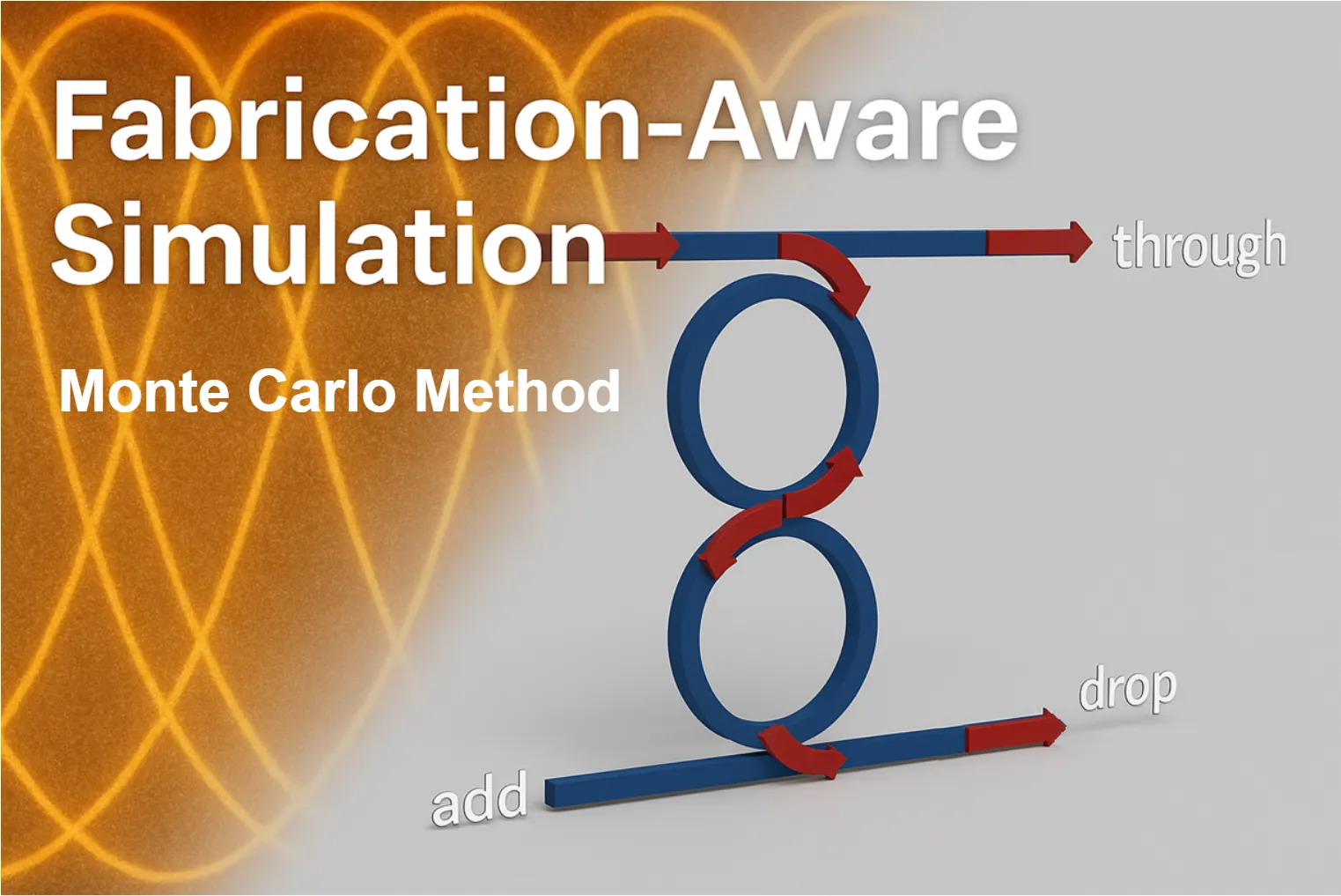
In this notebook we demonstrate how we can perform fabrication-aware simulations in PhotonForge by modeling a 2-ring coupled resonator filter and running a Monte Carlo analysis on key process-variation parameters. We focus on variations in the coupler gap, silicon wafer thickness, and sidewall angle, then visualize their impact on spectral response.

We use the couple mode theory presented in [1] for the filter design.

References

1. Little, Brent E., et al. “Microring resonator channel dropping filters.” Journal of lightwave technology 1997 15 (6), 998-1005, doi: 10.1109/50.588673.

import matplotlib.pyplot as plt
import numpy as np
import pandas as pd
import photonforge as pf
import tidy3d as td
from scipy.signal import find_peaks

# Reduce non-critical Tidy3D logs to keep the notebook output clean
td.config.logging.level = "ERROR"

Setting Up Technology and Simulation Defaults

Here we load and configure the default technology, mesh, and wavelength settings that will be used throughout the notebook.
We start from PhotonForge’s basic technology, set it as the default, and define a bending radius and port specification. We also fix a mesh refinement level and specify the simulation wavelength range around 1.55 µm — the telecom C-band region where most silicon photonic devices operate.

# Load the basic technology
tech = pf.basic_technology()

# Set this as the default technology for all subsequent components
pf.config.default_technology = tech

# Extract the standard single-mode strip waveguide port specification
port_spec = tech.ports["Strip"]

# Set some default parameters for all components (e.g., bend radius)
pf.config.default_kwargs = {
    "radius": 5,  # bend radius in microns
    "port_spec": port_spec,
}

# Define the default mesh refinement level
pf.config.default_mesh_refinement = 15

# Define the wavelength range for optical simulations [µm]
wavelengths = np.linspace(1.543, 1.557, 401)

Parametric 2-Ring Filter Construction

We define a parametric function to build a two coupled ring resonator (2-RR) filter using PhotonForge primitives. The function instantiates two types of couplers — a bus-to-ring coupler and a ring-to-ring coupler — and then stitches them with a netlist that sets up instances, interconnects ports, and exposes the device I/O.

What we parameterize

• coupling_length: the straight interaction length in the couplers, controlling the coupling coefficient.
• bus_coupling_distance: the nominal gap between the bus waveguide and each ring.
• ring_coupling_distance: the nominal gap between the two rings in the inter-ring coupler.

Netlist assembly We instantiate:

• Two bus couplers (bus_coupler0, bus_coupler1)
• One ring-to-ring coupler (ring_coupler0)

We then connect their ports to form the 2-RR filter topology and publish four external ports.

Finally, we build the component from the netlist and create a default instance for quick visualization.

Flat-Top (Maximally-Flat) Design Condition

To achieve a flat-top (maximally-flat) passband in the two-ring add–drop filter (with identical rings), we choose the coupling gaps such that the bus-to-ring and ring-to-ring coupling coefficients satisfy the synthesis relation derived in [1]:

$\kappa_{\text{int}} = \frac{1}{2} \kappa_{\text{ext}}^2$

where:

• $\kappa_{\text{ext}}$ — bus-to-ring (external) power coupling coefficient ($\kappa_{\text{ext}} \approx 0.4$ in our design)
• $\kappa_{\text{int}}$ — ring-to-ring (internal) power coupling coefficient ($\kappa_{\text{int}} \approx 0.08$ in our design)

This condition ensures a maximally-flat spectral response by properly balancing external and internal coupling strengths.

@pf.parametric_component
def create_two_rr_filter(
    *,
    coupling_length: float = 13.5,
    bus_coupling_distance: float = 0.7,
    ring_coupling_distance: float = 0.81,
) -> pf.Component:
    """
    Build a 2-ring (2RR) filter from parametric couplers and return the component.
    """
    # Parametric subcomponents
    bus_to_ring = pf.parametric.dual_ring_coupler(
        coupling_distance=bus_coupling_distance,
        coupling_length=coupling_length,
        model=pf.Tidy3DModel(
            verbose=False,
            port_symmetries=[
                ("P1", "P0", "P3", "P2"),
                ("P2", "P3", "P0", "P1"),
                ("P3", "P2", "P1", "P0"),
            ],
        ),
    )

    ring_to_ring = bus_to_ring.copy().update(coupling_distance=ring_coupling_distance)

    # Netlist for assembling the 2RR resonator
    netlist_2RR = {
        "name": "filter",
        "instances": {
            "bus_coupler0": bus_to_ring,
            "bus_coupler1": bus_to_ring,
            "ring_coupler0": ring_to_ring,
        },
        "connections": [
            (("ring_coupler0", "P0"), ("bus_coupler0", "P1")),
            (("bus_coupler1", "P3"), ("ring_coupler0", "P1")),
        ],
        "ports": [
            ("bus_coupler0", "P0"),
            ("bus_coupler1", "P2"),
            ("bus_coupler0", "P2"),
            ("bus_coupler1", "P0"),
        ],
        "models": [pf.CircuitModel()],
    }

    two_rr = pf.component_from_netlist(netlist_2RR)
    return two_rr

two_rr = create_two_rr_filter()
two_rr

LayoutSchematic

We now compute and visualize the spectral characteristics of the designed 2-RR filter.

# Compute the scattering matrix (S-matrix) of the 2RR filter across wavelengths
s_matrix_2rr = two_rr.s_matrix(frequencies=pf.C_0 / wavelengths)

# Plot the S-matrix with input from port P0, showing response in dB
_ = pf.plot_s_matrix(s_matrix_2rr, input_ports=["P0"])

Uploading task 'Mode-Stripwaveguide…'
Uploading task 'Mode-Stripwaveguide…'
Starting task 'Mode-Stripwaveguide': https://tidy3d.simulation.cloud/workbench?taskId=mo-b12b7575-2179-4168-9528-9d1d338cb5e4
Downloading data from 'Mode-Stripwaveguide'…
Starting task 'Mode-Stripwaveguide': https://tidy3d.simulation.cloud/workbench?taskId=mo-c8f0fbf1-c784-4e0a-8eb8-b3b610131f30
Downloading data from 'Mode-Stripwaveguide'…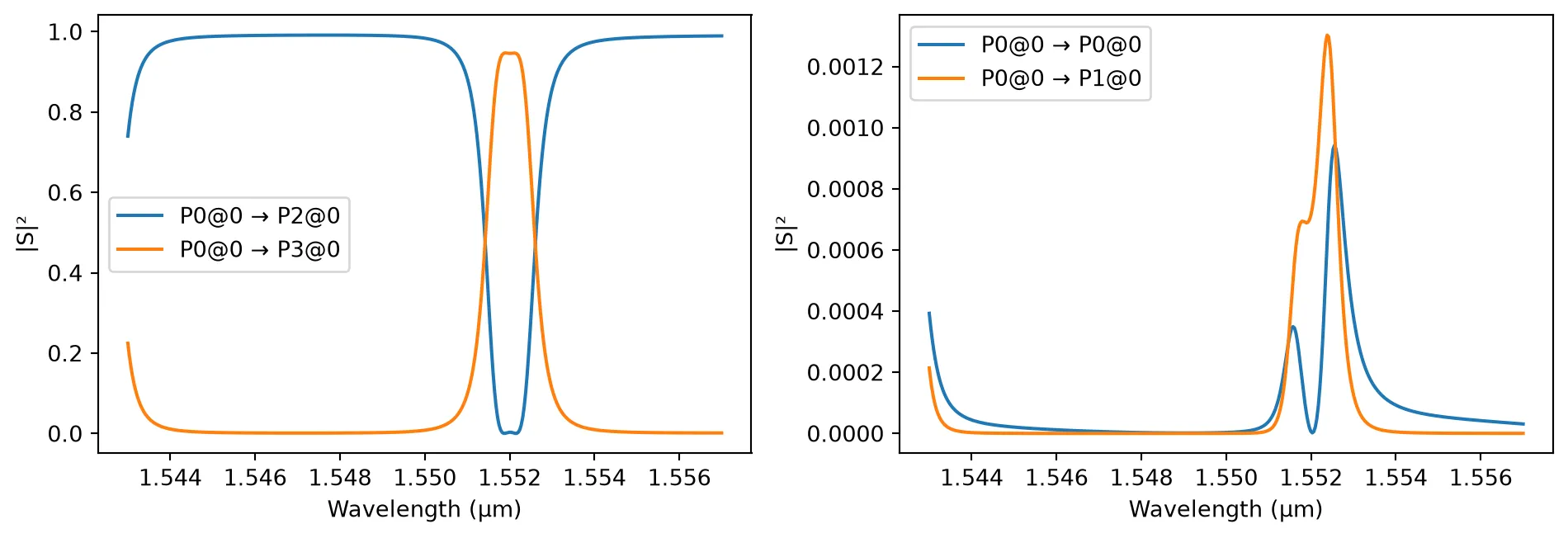

Monte Carlo Analysis

To evaluate fabrication tolerance and yield, we perform a Monte Carlo simulation on the 2-RR filter.
Each sample randomly perturbs selected geometric and material parameters within specified distributions, emulating real-world process variations.

Parameters under variation

• core_thickness (technology): silicon layer thickness, mean 0.22 µm with a 3 nm standard deviation
• sidewall_angle (technology): etched sidewall deviation, uniformly sampled between 0° and 5°
• bus_coupling_distance (component): coupling gap between bus and ring, mean 0.7 µm with 10 nm σ
• ring_coupling_distance (component): gap between rings, mean 0.79 µm with 10 nm σ

We include both random and corner samples to span statistical variability and worst-case scenarios.
The resulting dataset contains a list of parameter realizations and their corresponding S-matrices.

# Run a Monte Carlo S-matrix analysis to capture fabrication-induced variations
var, results = pf.monte_carlo.s_matrix(
    two_rr,
    pf.C_0 / wavelengths,
    ("core_thickness", "technology", {"value": 0.22, "stdev": 0.003}),
    ("sidewall_angle", "technology", {"value_range": [0, 5]}),
    ("bus_coupling_distance", two_rr, {"value": 0.7, "stdev": 0.01}),
    ("ring_coupling_distance", two_rr, {"value": 0.81, "stdev": 0.01}),
    random_samples=20,  # number of random samples
    corner_samples=2,  # corner cases (extreme combinations)
    random_seed=0,
    show_progress=True,
)

Starting sample 1 of 22…
Uploading task 'Mode-Stripwaveguide…'
Uploading task 'Mode-Stripwaveguide…'
Starting sample 2 of 22…
Uploading task 'Mode-Stripwaveguide…'
Uploading task 'Mode-Stripwaveguide…'
Starting sample 3 of 22…
Uploading task 'Mode-Stripwaveguide…'
Uploading task 'Mode-Stripwaveguide…'
Starting sample 4 of 22…
Starting task 'Mode-Stripwaveguide': https://tidy3d.simulation.cloud/workbench?taskId=mo-5102f988-67c8-4c6b-b353-9989c2956796
Uploading task 'Mode-Stripwaveguide…'
Uploading task 'Mode-Stripwaveguide…'
Starting task 'Mode-Stripwaveguide': https://tidy3d.simulation.cloud/workbench?taskId=mo-3eb49050-be8d-4a88-9ad8-ab347e712dd2
Starting task 'Mode-Stripwaveguide': https://tidy3d.simulation.cloud/workbench?taskId=mo-cbf26adb-4dcf-421f-abcf-9d494c35b7ce
Starting sample 5 of 22…
Starting task 'Mode-Stripwaveguide': https://tidy3d.simulation.cloud/workbench?taskId=mo-4a5ac660-f330-44f6-b8d5-983f8f282e67
Starting task 'Mode-Stripwaveguide': https://tidy3d.simulation.cloud/workbench?taskId=mo-4aad1484-a714-4c24-969b-12211563bb5d
Uploading task 'Mode-Stripwaveguide…'
Downloading data from 'Mode-Stripwaveguide'…
Uploading task 'Mode-Stripwaveguide…'
Starting sample 6 of 22…
Downloading data from 'Mode-Stripwaveguide'…
Downloading data from 'Mode-Stripwaveguide'…
Downloading data from 'Mode-Stripwaveguide'…
Starting task 'Mode-Stripwaveguide': https://tidy3d.simulation.cloud/workbench?taskId=mo-530ab37e-e754-4968-b197-2f151f4174e7
Downloading data from 'Mode-Stripwaveguide'…
Uploading task 'Mode-Stripwaveguide…'
Uploading task 'Mode-Stripwaveguide…'
Starting task 'Mode-Stripwaveguide': https://tidy3d.simulation.cloud/workbench?taskId=mo-7197e494-4f9d-46d6-b2be-fa763bea671e
Starting sample 7 of 22…
Downloading data from 'Mode-Stripwaveguide'…
Uploading task 'Mode-Stripwaveguide…'
Uploading task 'Mode-Stripwaveguide…'
Starting task 'Mode-Stripwaveguide': https://tidy3d.simulation.cloud/workbench?taskId=mo-316c774b-b014-482d-a18d-e534ba1d5170
Starting task 'Mode-Stripwaveguide': https://tidy3d.simulation.cloud/workbench?taskId=mo-0b09ba58-1d0d-4bdc-a97a-d356016f0f8e
Starting sample 8 of 22…
Downloading data from 'Mode-Stripwaveguide'…
Uploading task 'Mode-Stripwaveguide…'
Uploading task 'Mode-Stripwaveguide…'
Starting sample 9 of 22…
Starting task 'Mode-Stripwaveguide': https://tidy3d.simulation.cloud/workbench?taskId=mo-1738f11a-c838-4d74-8b9c-0b61e9a78b16
Starting task 'Mode-Stripwaveguide': https://tidy3d.simulation.cloud/workbench?taskId=mo-505428ef-45d8-41b0-8eaa-86039bf22630
Downloading data from 'Mode-Stripwaveguide'…
Starting task 'Mode-Stripwaveguide': https://tidy3d.simulation.cloud/workbench?taskId=mo-f5536116-9e9e-4381-a84f-6538ba76decb
Uploading task 'Mode-Stripwaveguide…'
Uploading task 'Mode-Stripwaveguide…'
Downloading data from 'Mode-Stripwaveguide'…
Starting sample 10 of 22…
Starting task 'Mode-Stripwaveguide': https://tidy3d.simulation.cloud/workbench?taskId=mo-9bb52ad8-afa1-4f4d-b73d-003ccb64c54c
Uploading task 'Mode-Stripwaveguide…'
Uploading task 'Mode-Stripwaveguide…'
Starting task 'Mode-Stripwaveguide': https://tidy3d.simulation.cloud/workbench?taskId=mo-9eed98f0-bafb-4fcc-9afe-4b8009e48a51
Downloading data from 'Mode-Stripwaveguide'…
Downloading data from 'Mode-Stripwaveguide'…
Downloading data from 'Mode-Stripwaveguide'…
Starting task 'Mode-Stripwaveguide': https://tidy3d.simulation.cloud/workbench?taskId=mo-52a0d4fa-0485-4459-b133-9f483a00a160
Starting sample 11 of 22…
Starting task 'Mode-Stripwaveguide': https://tidy3d.simulation.cloud/workbench?taskId=mo-6a3faba3-ee06-4a05-9e27-1d5e83d0383c
Uploading task 'Mode-Stripwaveguide…'
Downloading data from 'Mode-Stripwaveguide'…
Uploading task 'Mode-Stripwaveguide…'
Downloading data from 'Mode-Stripwaveguide'…
Starting task 'Mode-Stripwaveguide': https://tidy3d.simulation.cloud/workbench?taskId=mo-c5e133a0-6a7d-4705-ab01-a513eacac260
Starting sample 12 of 22…
Downloading data from 'Mode-Stripwaveguide'…
Starting task 'Mode-Stripwaveguide': https://tidy3d.simulation.cloud/workbench?taskId=mo-2653da79-c59d-4d2f-9ef8-e36a162e1331
Downloading data from 'Mode-Stripwaveguide'…
Uploading task 'Mode-Stripwaveguide…'
Uploading task 'Mode-Stripwaveguide…'
Starting task 'Mode-Stripwaveguide': https://tidy3d.simulation.cloud/workbench?taskId=mo-a0d416ab-7f01-40ee-9bbc-46cc3868d008
Starting task 'Mode-Stripwaveguide': https://tidy3d.simulation.cloud/workbench?taskId=mo-354c6c6f-e2a5-4637-bd62-716b1eb64e66
Downloading data from 'Mode-Stripwaveguide'…
Starting sample 13 of 22…
Downloading data from 'Mode-Stripwaveguide'…
Starting task 'Mode-Stripwaveguide': https://tidy3d.simulation.cloud/workbench?taskId=mo-6a9ce0f8-f9ea-47e9-bdcc-a53ff044fc5b
Starting task 'Mode-Stripwaveguide': https://tidy3d.simulation.cloud/workbench?taskId=mo-f273c9dc-a06d-4e06-ac2c-6a7cc07c468a
Downloading data from 'Mode-Stripwaveguide'…
Uploading task 'Mode-Stripwaveguide…'
Uploading task 'Mode-Stripwaveguide…'
Downloading data from 'Mode-Stripwaveguide'…
Starting task 'Mode-Stripwaveguide': https://tidy3d.simulation.cloud/workbench?taskId=mo-d3e6475c-eb03-4dda-b239-4ffff9c411b5
Starting sample 14 of 22…
Starting task 'Mode-Stripwaveguide': https://tidy3d.simulation.cloud/workbench?taskId=mo-c2259f48-ef93-4ed3-b304-841e19b4d537
Downloading data from 'Mode-Stripwaveguide'…
Downloading data from 'Mode-Stripwaveguide'…
Downloading data from 'Mode-Stripwaveguide'…
Uploading task 'Mode-Stripwaveguide…'
Uploading task 'Mode-Stripwaveguide…'
Starting task 'Mode-Stripwaveguide': https://tidy3d.simulation.cloud/workbench?taskId=mo-dc9f8057-9880-4044-9b5d-48abcefe045b
Starting task 'Mode-Stripwaveguide': https://tidy3d.simulation.cloud/workbench?taskId=mo-05c39506-726e-42c5-953f-0cc80efaff60
Downloading data from 'Mode-Stripwaveguide'…
Starting sample 15 of 22…
Downloading data from 'Mode-Stripwaveguide'…
Uploading task 'Mode-Stripwaveguide…'
Uploading task 'Mode-Stripwaveguide…'
Starting task 'Mode-Stripwaveguide': https://tidy3d.simulation.cloud/workbench?taskId=mo-1afdb9cc-f924-4064-8098-8a0e5035cc9e
Downloading data from 'Mode-Stripwaveguide'…
Starting task 'Mode-Stripwaveguide': https://tidy3d.simulation.cloud/workbench?taskId=mo-b5a8fcba-87e2-4c86-8167-cc1ee94274b6
Starting sample 16 of 22…
Downloading data from 'Mode-Stripwaveguide'…
Uploading task 'Mode-Stripwaveguide…'
Uploading task 'Mode-Stripwaveguide…'
Starting sample 17 of 22…
Downloading data from 'Mode-Stripwaveguide'…
Uploading task 'Mode-Stripwaveguide…'
Starting task 'Mode-Stripwaveguide': https://tidy3d.simulation.cloud/workbench?taskId=mo-ce693e10-b5d3-41e8-91c5-8f3ec88a5063
Uploading task 'Mode-Stripwaveguide…'
Starting task 'Mode-Stripwaveguide': https://tidy3d.simulation.cloud/workbench?taskId=mo-9a66d67a-a9f5-4337-87c6-a1d7516e9b85
Starting sample 18 of 22…
Downloading data from 'Mode-Stripwaveguide'…
Downloading data from 'Mode-Stripwaveguide'…
Starting task 'Mode-Stripwaveguide': https://tidy3d.simulation.cloud/workbench?taskId=mo-26103914-06e4-4f8e-aeb4-e7dd433ee5ab
Starting task 'Mode-Stripwaveguide': https://tidy3d.simulation.cloud/workbench?taskId=mo-1d43586e-f826-4c20-93a6-b43505ebd819
Uploading task 'Mode-Stripwaveguide…'
Uploading task 'Mode-Stripwaveguide…'
Starting task 'Mode-Stripwaveguide': https://tidy3d.simulation.cloud/workbench?taskId=mo-b0c89d19-30eb-46d6-b67f-c498a90c17cb
Starting task 'Mode-Stripwaveguide': https://tidy3d.simulation.cloud/workbench?taskId=mo-a769e1fc-4520-470f-bc2c-1044e011db3b
Starting sample 19 of 22…
Downloading data from 'Mode-Stripwaveguide'…
Downloading data from 'Mode-Stripwaveguide'…
Uploading task 'Mode-Stripwaveguide…'
Uploading task 'Mode-Stripwaveguide…'
Downloading data from 'Mode-Stripwaveguide'…
Starting sample 20 of 22…
Starting task 'Mode-Stripwaveguide': https://tidy3d.simulation.cloud/workbench?taskId=mo-79948aca-0c37-49a0-a525-c2daf9f0535e
Uploading task 'Mode-Stripwaveguide…'
Downloading data from 'Mode-Stripwaveguide'…
Uploading task 'Mode-Stripwaveguide…'
Starting task 'Mode-Stripwaveguide': https://tidy3d.simulation.cloud/workbench?taskId=mo-4a4dd394-49e0-4695-abb3-89927b45da79
Starting task 'Mode-Stripwaveguide': https://tidy3d.simulation.cloud/workbench?taskId=mo-b76514eb-0278-40c0-b2fe-5e6d2580cd50
Starting sample 21 of 22…
Starting task 'Mode-Stripwaveguide': https://tidy3d.simulation.cloud/workbench?taskId=mo-4b54f085-c973-45f6-80f8-4a547919840f
Downloading data from 'Mode-Stripwaveguide'…
Uploading task 'Mode-Stripwaveguide…'
Uploading task 'Mode-Stripwaveguide…'
Downloading data from 'Mode-Stripwaveguide'…
Downloading data from 'Mode-Stripwaveguide'…
Starting task 'Mode-Stripwaveguide': https://tidy3d.simulation.cloud/workbench?taskId=mo-607acdd6-4d11-4dad-a0d7-9e3e4ad9b6ea
Starting sample 22 of 22…
Starting task 'Mode-Stripwaveguide': https://tidy3d.simulation.cloud/workbench?taskId=mo-017fb79c-f808-4b59-87c9-f33f0ad7e73b
Uploading task 'Mode-Stripwaveguide…'
Downloading data from 'Mode-Stripwaveguide'…
Uploading task 'Mode-Stripwaveguide…'
Downloading data from 'Mode-Stripwaveguide'…
Starting task 'Mode-Stripwaveguide': https://tidy3d.simulation.cloud/workbench?taskId=mo-3bf4804e-bfde-465d-8ead-04cac076771f
Sample 1 done.
Sample 2 done.
Sample 3 done.
Sample 4 done.
Sample 5 done.
Sample 6 done.
Sample 7 done.
Sample 8 done.
Sample 9 done.
Sample 10 done.
Sample 11 done.
Sample 12 done.
Sample 13 done.
Sample 14 done.
Sample 15 done.
Sample 17 done.
Downloading data from 'Mode-Stripwaveguide'…
Starting task 'Mode-Stripwaveguide': https://tidy3d.simulation.cloud/workbench?taskId=mo-09588c65-ca4a-4eba-a8c6-9cffaa20f120
Sample 16 done.
Sample 18 done.
Downloading data from 'Mode-Stripwaveguide'…
Downloading data from 'Mode-Stripwaveguide'…
Starting task 'Mode-Stripwaveguide': https://tidy3d.simulation.cloud/workbench?taskId=mo-8b8c66c8-0cac-4121-ad6e-b008e3ab8618
Starting task 'Mode-Stripwaveguide': https://tidy3d.simulation.cloud/workbench?taskId=mo-e0489b70-959a-4333-9709-60b520ae19c5
Downloading data from 'Mode-Stripwaveguide'…
Downloading data from 'Mode-Stripwaveguide'…
Sample 19 done.
Sample 20 done.
Sample 22 done.
Sample 21 done.
All samples done!

We now plot the transmission spectra from port P0 (input) to port P3 (drop port) for all Monte Carlo samples.
Each curve represents one possible fabricated instance of the 2-RR filter, allowing us to observe the spread in resonance wavelength and insertion loss due to process variations.

fig, ax = plt.subplots(1, 1)

for *_, s_matrix in results:
    ax.plot(
        s_matrix.wavelengths,
        20 * np.log10(np.abs(s_matrix[("P0@0", "P3@0")])),
        alpha=0.5,
        color="tab:orange",
    )

_ = ax.set(ylim=(-20, 0), xlabel="λ (µm)", ylabel="Transmission (dB)")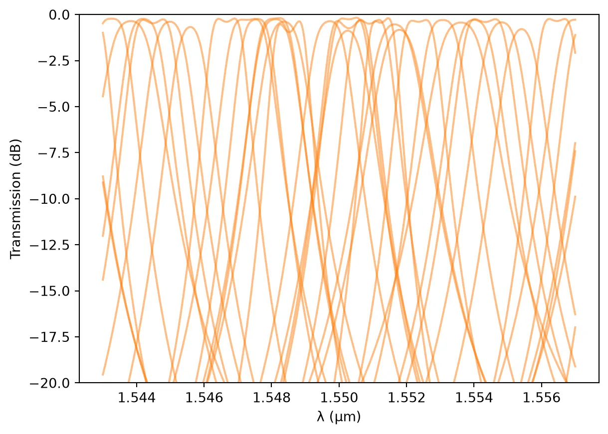

Discussion of Fabrication-Aware Results

The Monte Carlo simulation shows that fabrication variations can significantly impact the spectral response of the 2-RR filter:

• Resonance wavelength drift:
  The resonance positions vary substantially between samples, indicating that small deviations in silicon thickness, sidewall angle, or coupling gaps lead to noticeable phase shifts and effective index changes.
  This explains why thermal tuning (via integrated heaters) is almost always required in fabricated ring filters to fine-tune or align the resonance wavelengths post-fabrication.

• Insertion loss variation:
  The simulated through-port transmission fluctuates between approximately 0.3 dB and 1.0 dB, demonstrating that while loss performance changes slightly, the filter remains fairly robust to process deviations in this respect.

Overall, the analysis illustrates how PhotonForge’s fabrication-aware modeling can predict both resonance misalignment and performance spread, allowing designers to anticipate tuning requirements and optimize yield.

Correlation Analysis

Monte Carlo analysis allows for the extraction of correlations between a device’s response and its input variables. This section demonstrates the correlation analysis process. Critically, accurate results with four input variables require hundreds of data points. The findings presented here are, therefore, purely illustrative and not statistically significant.

Feature extraction

In this section we extract three filter features from each simulated S-matrix so we can study their correlation with fabrication variables. We target the resonance closest to a reference wavelength $\lambda_0$ (default $1.55 \mu$m) and compute:

• Center wavelength $\lambda_c$: the midpoint between the two 3-dB crossing wavelengths around the chosen resonance.
• Insertion loss IL (in dB): transmission value at the center wavelength.
• 3-dB bandwidth $\Delta\lambda_{3,\text{dB}}$: difference between the right and left 3-dB crossing wavelengths.

def extract_filter_features(s_matrix, target_wavelength=1.55):
    """
    Extracts key features (insertion loss, center wavelength, bandwidth)
    from an optical filter's S-matrix data.

    This function identifies the resonance dip closest to a target wavelength
    and calculates its characteristics.

    Args:
        s_matrix: The S-matrix object from the simulation.
        target_wavelength (float): The wavelength (in µm) around which to
                                   search for the primary resonance.
                                   Defaults to 1.55 µm.

    Returns:
        dict: A dictionary containing the calculated 'center_wavelength',
              'insertion_loss' (in dB), and 'bandwidth' (in µm).
              Returns None if no resonance is found.
    """
    wavelengths = s_matrix.wavelengths
    # Calculate transmission in dB
    transmission_db = 20 * np.log10(np.abs(s_matrix[("P0@0", "P3@0")]))

    # The 'prominence' parameter helps ignore minor ripples and noise.
    peak_indices, _ = find_peaks(transmission_db, prominence=1)

    if peak_indices.size == 0:
        print("Warning: No resonance peaks found.")
        return None

    # Find the peak/resonance closest to the target wavelength
    resonant_wavelengths = wavelengths[peak_indices]
    closest_peak_index = peak_indices[
        np.argmin(np.abs(resonant_wavelengths - target_wavelength))
    ]

    # --- 1. Calculate Maximum Transmission Wavelength and Insertion Loss ---
    max_wavelength = wavelengths[closest_peak_index]
    insertion_loss = transmission_db[closest_peak_index]

    # --- 2. Calculate 3-dB Bandwidth ---
    # The 3-dB level is 3 dB below the maximum transmission value (the IL)
    three_db_level = insertion_loss - 3

    # Find where the transmission crosses the 3-dB level on both sides of the resonance
    # Split the transmission data at the resonance point
    left_side = transmission_db[:closest_peak_index]
    right_side = transmission_db[closest_peak_index:]

    # Find the indices where the transmission is greater than the 3-dB level
    left_indices_below_3db = np.where(left_side < three_db_level)[0]
    right_indices_below_3db = np.where(right_side < three_db_level)[0]

    if left_indices_below_3db.size == 0 or right_indices_below_3db.size == 0:
        bandwidth = np.nan  # Use NaN for cases where bandwidth can't be found
    else:
        # Get the points just before and after the crossing
        left_cross_idx = left_indices_below_3db[-1]
        right_cross_idx = right_indices_below_3db[0] + closest_peak_index

        # Interpolate to find the exact wavelength at the 3dB crossing for better accuracy
        w_left = np.interp(
            three_db_level,
            [transmission_db[left_cross_idx], transmission_db[left_cross_idx + 1]],
            [wavelengths[left_cross_idx], wavelengths[left_cross_idx + 1]],
        )

        w_right = np.interp(
            three_db_level,
            [transmission_db[right_cross_idx - 1], transmission_db[right_cross_idx]],
            [wavelengths[right_cross_idx - 1], wavelengths[right_cross_idx]],
        )

        # Compute bandwidth and center wavelength from crossings
        bandwidth = w_right - w_left
        center_wavelength = (w_right + w_left) / 2
        insertion_loss = transmission_db[(left_cross_idx + right_cross_idx) // 2]

    return {
        "center_wavelength": center_wavelength,
        "insertion_loss": insertion_loss,
        "bandwidth": bandwidth,
    }

Correlation Matrix

In this section we take the Monte Carlo results and visually explore how each fabrication parameter affects the main filter features.
We generate a grid of scatter plots, one for each input–output pair, annotated with the Pearson correlation coefficient (R).

Interpretation

• R ≈ +1: Strong positive correlation — as the fabrication parameter increases, the feature value increases.
• R ≈ -1: Strong negative correlation — the feature decreases as the parameter increases.
• R ≈ 0: Weak or no linear correlation.

This visualization allows us to directly identify which fabrication tolerances most strongly impact spectral behavior such as resonance shift, insertion loss, or bandwidth broadening.

Important note: The correlation results shown here are intended for demonstration only and are not statistically valid because of small number of data points.

def run_correlation_analysis(variables, simulation_results, target_wavelength=1.55):
    """
    Processes Monte Carlo simulation results to visualize the relationship
    and correlation between each input variable and each output filter feature.

    Args:
        variables (list): The list of RandomVariable objects from the simulation.
        simulation_results (list): The list of result tuples from the simulation.
                                     Each tuple contains the input values and the s_matrix.
        target_wavelength (float): The target wavelength in micrometers.
    """
    data = []
    variable_names = [v.name for v in variables]

    print("Processing simulation results...")
    for result in simulation_results:
        s_matrix = result[-1]
        input_values = result[:-1]
        features = extract_filter_features(
            s_matrix, target_wavelength=target_wavelength
        )

        if features:
            run_data = {name: val for name, val in zip(variable_names, input_values)}
            run_data.update(features)
            data.append(run_data)

    if not data:
        print("Could not extract features from any simulation run. Aborting.")
        return

    print(f"Successfully processed {len(data)} data points.")
    df = pd.DataFrame(data)
    df["center_wavelength"] *= 1e3
    df["bandwidth"] *= 1e3
    df = df.rename(
        columns={
            "center_wavelength": "center_wavelength_nm",
            "bandwidth": "bandwidth_nm",
        }
    )

    print("\n--- Data Head ---")
    print(df.head())

    output_feature_names = ["insertion_loss", "center_wavelength_nm", "bandwidth_nm"]

    print("\n--- Generating Custom Scatter Plot Grid with Correlation Values ---")

    n_outputs = len(output_feature_names)
    n_inputs = len(variable_names)

    fig, axes = plt.subplots(
        n_outputs, n_inputs, figsize=(10, 8), sharex="col", sharey="row"
    )

    if n_outputs == 1 or n_inputs == 1:
        axes = np.array(axes).reshape(n_outputs, n_inputs)

    for i, out_feature in enumerate(output_feature_names):
        for j, in_variable in enumerate(variable_names):
            ax = axes[i, j]
            ax.scatter(
                df[in_variable],
                df[out_feature],
                alpha=0.6,
                s=30,
                edgecolor="k",
                linewidth=0.5,
            )
            corr = df[in_variable].corr(df[out_feature])
            corr_text = f"R = {corr:.2f}"
            ax.text(
                0.05,
                0.95,
                corr_text,
                transform=ax.transAxes,
                fontsize=12,
                verticalalignment="top",
                bbox=dict(boxstyle="round,pad=0.3", facecolor="wheat", alpha=0.5),
            )
            if j == 0:
                ax.set_ylabel(out_feature, fontsize=12)
            if i == n_outputs - 1:
                ax.set_xlabel(in_variable, fontsize=12)

            ax.tick_params(axis="x", rotation=45)
            ax.grid(True, linestyle="--", alpha=0.6)

    fig.suptitle("Output Features vs. Input Variables", fontsize=20)
    plt.tight_layout(rect=[0, 0.03, 1, 0.97])
    plt.show()

run_correlation_analysis(var, results)

Processing simulation results...
Successfully processed 22 data points.

--- Data Head ---
   sidewall_angle  core_thickness  ring_coupling_distance  \
0        5.000000        0.225880                0.829600
1        0.000000        0.214120                0.790400
2        4.517759        0.218700                0.817602
3        4.244655        0.219547                0.792679
4        2.785838        0.219909                0.808466

   bus_coupling_distance  center_wavelength_nm  insertion_loss  bandwidth_nm
0               0.719600           1551.269666       -0.437801      0.960668
1               0.680400           1553.621434       -0.432439      1.577132
2               0.699238           1549.720321       -0.360124      1.189357
3               0.713226           1550.306584       -0.744145      1.416833
4               0.703479           1548.111936       -0.212000      1.256127

--- Generating Custom Scatter Plot Grid with Correlation Values ---