FMCW Ranging with the LiDAR Chip

Download notebook (.zip)

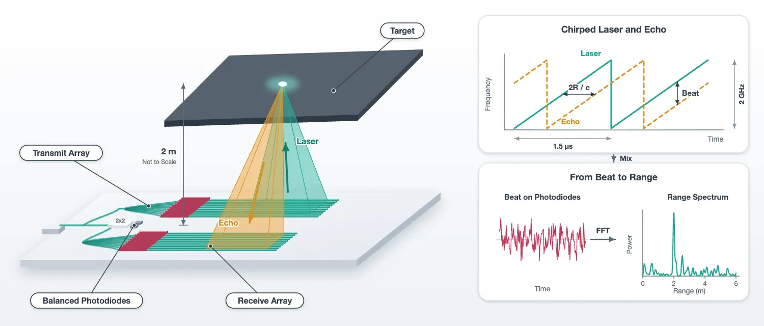
This page drives the chip of the layout page with a chirped laser and reads range and speed from the beat on its balanced photodiodes. It does five things:

It assembles the full link budget from the losses, the antenna efficiency and the beam pattern measured on the earlier pages, and computes the detection range.
It puts the chip into PhotonForge’s circuit time stepper and checks the stepped chip against its S matrix.
It models the space between the two arrays: the transmitted beam, the target, the return.
It measures range, speed, range resolution, the effect of laser linewidth, and the signal to noise against range, each against the budget.
It steers the beam with the heater settings of the steering page and builds a range image of a scene with six targets.

The chip enters the simulation in two places. On the transmit side its S matrix, from the layout, sets the amplitude and phase of the light at each antenna. On the receive side the chip is stepped in time: the returned fields enter its 32 receive ports, the laser enters its fibre port, and the time stepper produces the two photodiode voltages.

The chirp bandwidth is 2 GHz, as the budget set. The chirp lasts 1.5 us on this page instead of the 10 us of the budget. The range resolution depends only on the bandwidth. The shorter chirp cuts the number of time steps by seven. The chirp duration enters the signal-to-noise ratio, and there the budget is scaled to the simulated record length.

# Everything before this page: the technology, the antennas, the components, the layout, the
# steering table and the beam functions
from runpy import run_path

# Lidar_Steering.qmd defines what this notebook builds on. Its shared cells are
# generated into the module below; see docs/scripts/generate_notebook_modules.py.
globals().update(
    {k: v for k, v in run_path("misc/lidar_steering.py").items() if not k.startswith("_")}
)

from photonforge.live_viewer import LiveViewer

# Layout viewer for the chip driven below
viewer = LiveViewer()

q_e = 1.602e-19  # Elementary charge (C), for the threshold current of the DM laser
z0 = 50.0  # Impedance of the electrical ports: voltage = wave amplitude x sqrt(z0)
# Time step (s): a 25 GHz band, twelve times the chirp bandwidth; one delay step is 3 mm of range
dt = 20e-12
t_sim = 1.5e-6  # Duration of one chirp ramp on this page (s)
# Time discarded at the start of every run: the longest round trip and the photodiode filter (s)
t_settle = 100e-9
n_settle = int(round(t_settle / dt))
slope = b_chirp / t_sim  # Chirp rate (Hz/s)
print(
    f"chirp {b_chirp * 1e-9:.0f} GHz in {t_sim * 1e6:.1f} us: {slope * 1e-12:.0f} MHz per us, "
    f"beat {2 * slope / c0 * 1e-6:.1f} MHz per metre of range"
)

LiveViewer started at http://127.0.0.1:37443. Call its 'stop()' method to free the port.
chirp 2 GHz in 1.5 us: 1333 MHz per us, beat 8.9 MHz per metre of range

The link budget

The transmit array radiates the power $P_\text{rad}$ into a beam with directivity $G$ . A target at range $R$ on the beam axis receives the irradiance

I = \frac{P_\text{rad}\, G}{4\pi R^2} .

A diffuse (Lambertian) target with reflectivity $\rho$ scatters this light into a hemisphere with radiance $L = \rho I / \pi$ . The receiver is coherent, so it collects one spatial mode. A single-mode antenna that looks at an extended source of radiance $L$ collects the power $L \lambda^2$ times its efficiency, whatever its aperture: a larger aperture sees a smaller patch of the target through a narrower beam, and the product of the two is constant. The power in the guided modes of the receive array is therefore

P_\text{rx} = \frac{\rho}{\pi}\,\frac{P_\text{rad}\,G}{4\pi R^2}\,\lambda^2\,\eta_\text{rx} .

With $G = 4\pi A\,\eta_\text{ap} / \lambda^2$ for an aperture of area $A$ , this is the $\rho A / \pi R^2$ of the technology page, with the aperture efficiency $\eta_\text{ap}$ and the loss chain $\eta_\text{rx}$ written out. Each factor is taken from a measurement:

Facet, tap and transmit tree. The S matrix of the drawn chip without its antennas gives the fraction of the fibre power that reaches the 32 antenna inputs. The three parts are listed separately: the edge coupler from the component page, the through port of the tap, and the splitter tree with its waveguides from the feed cell alone.
Antenna efficiency $\eta_\text{ant}$ , from the antenna page: the fraction radiated over the antenna length times the share that reaches the air. By reciprocity the same factor applies to the light collected on the way back.
Directivity $G$ , from the lateral beam pattern of the steering page, which contains the sidelobes and the element pattern, and the longitudinal lobe of the antenna page.
Receive tree and coupler. The receive tree is the same feed cell used backwards, so it has the tree loss but no facet and no tap. The 2x2 coupler adds its excess loss. Its split between the two photodiodes is not a loss, because balanced detection adds the two beats.
Polarization. A rough target depolarizes the light and the antennas receive one polarization, so half of the return is lost.
Speckle. The return from a rough target is a speckle field. The power coupled into one mode is exponentially distributed about the mean above: a fraction $x$ of the mean is exceeded with probability $e^{-x}$ . A 10 dB fade margin covers 90 percent of the shots.

With a strong local oscillator, coherent detection is limited by the shot noise of the local oscillator. The signal-to-noise ratio in one chirp of duration $T$ is then the number of returned photons detected during the chirp,

\mathrm{SNR} = \frac{\eta\, P_\text{rx}\, T}{h\nu} ,

with $\eta$ the quantum efficiency of the photodiodes.

# The chip without its antennas: the fan-in outputs are ports, which is how it is driven here
chip_feeds = assemble_chip(antennas=False, name="lidar_chip_feeds")
viewer(chip_feeds)

# Fraction of the fibre power that reaches the 32 transmit antenna inputs, from the layout's S matrix
s_chip = chip_feeds.s_matrix(
    [f0], model_kwargs={"inputs": ["FIBER"]}, show_progress=False
)
tx_amps = np.array([s_chip[("FIBER@0", f"TX{k}@0")][0] for k in range(n_ch)])
to_antennas = np.sum(np.abs(tx_amps) ** 2)

# Its three parts: the edge coupler's loss, the through port of the tap, and the feed cell alone
facet_loss = 10 ** (-ec.parametric_kwargs["insertion_loss"] / 10)
tap_through = abs(coef["P2"]) ** 2
s_feed = feed.s_matrix([f0], model_kwargs={"inputs": ["IN"]}, show_progress=False)
through_tree = np.sum(
    np.abs([s_feed[("IN@0", f"A{k}@0")][0] for k in range(n_ch)]) ** 2
)

# The 2x2 coupler's excess loss, from the component page's EME sweep
mixer_excess = 1 / total_22.max()

# Antenna efficiency from the antenna page: fraction radiated over the length times the share in the air
eta_ant = efficiency

def directivity(amps):
    """Directivity against the lateral angle for the given antenna amplitudes: the lateral
    pattern of the array, element pattern included, times the longitudinal lobe of one antenna.
    """
    # Lateral power pattern of the array against theta (deg), from the steering page
    lateral = beam(amps)
    psi = np.radians(theta)
    # Longitudinal lobe of the millimetre antenna against its emission angle in air
    ux_fine = np.linspace(u_peak - 0.02, u_peak + 0.02, 4001)
    lobe = longitudinal_lobe(l_antenna, ux_fine)
    theta_long = np.arcsin(n_oxide * ux_fine)
    # Total radiated power as the integral over solid angle, d(omega) = cos(psi) d(psi) d(theta)
    total = np.trapezoid(lateral * np.cos(psi), psi) * np.trapezoid(lobe, theta_long)
    # Directivity: 4 pi times the power per unit solid angle over the total
    return 4 * np.pi * lateral * lobe.max() / total

gain = directivity(steered(0.0))
g_peak = gain.max()
aperture = aperture_x * 1e-6 * l_antenna * 1e-6  # Transmit aperture (m^2)
eta_ap = g_peak * (lda0 * 1e-6) ** 2 / (4 * np.pi * aperture)
print(
    f"directivity of the broadside beam {10 * np.log10(g_peak):.1f} dBi; a uniform aperture of the same size "
    f"would give {10 * np.log10(4 * np.pi * aperture / (lda0 * 1e-6) ** 2):.1f} dBi: aperture efficiency {eta_ap:.2f}"
)

# The budget as a chain of factors, in dB
fade_margin_db = 10.0  # Speckle margin (dB): covers 90 percent of the realizations
polarization = 0.5  # One polarization received from a depolarizing target
lines = [
    ("laser at the fibre", 10 * np.log10(p_laser * 1e3), "dBm"),
    ("edge coupler (component page)", 10 * np.log10(facet_loss), "dB"),
    ("tap, through port (component page)", 10 * np.log10(tap_through), "dB"),
    (
        "transmit tree and waveguides (feed cell S matrix)",
        10 * np.log10(through_tree),
        "dB",
    ),
    (
        "   check: fibre to the antenna inputs, whole chip S matrix",
        10 * np.log10(to_antennas),
        "dB",
    ),
    ("antenna efficiency, transmit (antenna page)", 10 * np.log10(eta_ant), "dB"),
    (
        "beam directivity, broadside (steering and antenna pages)",
        10 * np.log10(g_peak),
        "dBi",
    ),
    ("antenna efficiency, receive", 10 * np.log10(eta_ant), "dB"),
    (
        "receive tree and waveguides (feed cell S matrix)",
        10 * np.log10(through_tree),
        "dB",
    ),
    ("2x2 coupler excess (component page)", 10 * np.log10(1 / mixer_excess), "dB"),
    ("polarization", 10 * np.log10(polarization), "dB"),
]
print(f"\n{'factor':62s} value")
for name, value, unit in lines:
    print(f"{name:62s} {value:6.2f} {unit}")

# Radiated power, and the receive chain from the antennas to the mixer
p_rad = p_laser * to_antennas * eta_ant
eta_rx = eta_ant * through_tree / mixer_excess * polarization
ranges = np.linspace(1, 40, 400)

def returned_power(rho, r, g=g_peak):
    """Power at the mixer from a Lambertian target of reflectivity rho at range r (m), lit by a
    beam of directivity g: the budget formula."""
    irradiance = p_rad * g / (4 * np.pi * r**2)
    radiance = rho / np.pi * irradiance
    return radiance * (lda0 * 1e-6) ** 2 * eta_rx

# Returned power at the design range, the shot-noise SNR over one 10 us chirp, and the range at 10 dB
print(
    f"\n{'target':12s} {'return at 10 m':>16s} {'SNR, 10 us':>12s} {'range at 10 dB':>16s} {'with 10 dB fade margin':>24s}"
)
for name, rho in (("dark, 10 %", rho_dark), ("wall, 80 %", rho_bright)):
    p_rx = returned_power(rho, ranges)
    snr_db = 10 * np.log10(quantum_efficiency * p_rx * t_chirp / (h_planck * f0))
    r_10 = np.interp(-snr_min, -snr_db, ranges)
    r_fade = np.interp(-(snr_min + fade_margin_db), -snr_db, ranges)
    print(
        f"{name:12s} {returned_power(rho, r_design) * 1e15:13.0f} fW {np.interp(r_design, ranges, snr_db):9.1f} dB "
        f"{r_10:14.1f} m {r_fade:22.1f} m"
    )

Uploading task 'Mode-StripwaveguideTE500nm…'
Uploading task 'Mode-StripwaveguideTE500nm…'
Uploading task 'Mode-StripwaveguideTE500nm…'
Starting task 'Mode-StripwaveguideTE500nm': https://tidy3d.simulation.cloud/workbench?taskId=mo-35a006bb-f066-474e-8558-7fa28293c493
Downloading data from 'Mode-StripwaveguideTE500nm'…
Starting task 'Mode-StripwaveguideTE500nm': https://tidy3d.simulation.cloud/workbench?taskId=mo-152ba955-3d58-4912-a927-980f66c36176
Downloading data from 'Mode-StripwaveguideTE500nm'…
Starting task 'Mode-StripwaveguideTE500nm': https://tidy3d.simulation.cloud/workbench?taskId=mo-4e9e90ff-dedb-4d68-b894-da9c42d787b5
Downloading data from 'Mode-StripwaveguideTE500nm'…
directivity of the broadside beam 53.1 dBi; a uniform aperture of the same size would give 53.6 dBi: aperture efficiency 0.88

factor                                                         value
laser at the fibre                                              10.00 dBm
edge coupler (component page)                                   -1.50 dB
tap, through port (component page)                              -0.46 dB
transmit tree and waveguides (feed cell S matrix)               -0.62 dB
   check: fibre to the antenna inputs, whole chip S matrix      -2.58 dB
antenna efficiency, transmit (antenna page)                     -3.55 dB
beam directivity, broadside (steering and antenna pages)        53.05 dBi
antenna efficiency, receive                                     -3.55 dB
receive tree and waveguides (feed cell S matrix)                -0.62 dB
2x2 coupler excess (component page)                             -0.15 dB
polarization                                                    -3.01 dB

target         return at 10 m   SNR, 10 us   range at 10 dB   with 10 dB fade margin
dark, 10 %               6 fW      -5.1 dB            1.8 m                    1.0 m
wall, 80 %              44 fW       4.0 dB            5.0 m                    1.6 m

The fibre-to-antenna line is the sum of its three parts, which is the check that the whole-chip S matrix and the component measurements agree. The receive tree is smaller than the transmit line because the receive path has no edge coupler and no tap: the return enters through the antennas and only passes the splitter tree, the phase shifters and the fan-in waveguides.

The aperture efficiency is what the estimate on the technology page left out. The sidelobes, the light that the element pattern sends outside the beam, and the decaying illumination along the antenna cost half a decibel of directivity together. With the measured loss chain the white wall is ranged at five and a half metres and the dark target at two, before the speckle margin. With the margin, one to two metres is what a 10 mW laser and a 42 um by 1 mm aperture buy. Chip-scale phased-array LiDARs in the literature reach similar ranges. The return is femtowatts: a white wall at three metres sends back about seven photons per 2 us chirp. A longer chirp, a larger aperture or more laser power each extend the range as the square root.

The chip in the time domain

The chip without its antennas has 68 ports and about 450 components, counting every bend. The circuit time stepper steps each component. That costs four milliseconds per time step, and one chirp would take a day. The response of the feed network, however, does not vary over a 2 GHz chirp: a tree of splitters and waveguides has a constant amplitude and a delay for every pair of ports. Over the 25 GHz band of the time stepper, each element of the feed’s S matrix is

S_{pq}(f) = c_{pq}\, e^{\,2\pi j f d_{pq}} ,

with a complex constant $c_{pq}$ and a delay $d_{pq}$ . The library’s pole_residue_fit extracts exactly this: with delays="auto" it estimates the delay of each element from the data, the feedthrough term is the constant, and it adds poles only where the data ask for them. The result goes to the feed’s time stepper. The two MMIs are treated the same way, with the delay set to zero, since their 0.8 ps is negligible against the 40 ps period of the band and the estimate is less accurate than the poles. Elements between ports on the same side of a block, its reflections and the coupling between its outputs, are more than 30 dB down and on this page could only add beats at zero range; they are left out of the fit, which halves the stepping time. The tap, the edge coupler and the photodiodes keep their own time steppers.

A continuous-wave run checks that nothing was lost: the stepped amplitude and phase at every transmit port has to agree with the S matrix. The same run gives the steady photodiode voltages, from which the local-oscillator power on each photodiode follows through the responsivity and the transimpedance gain.

One convention fixes every sign below. The time stepper works in the rotating frame of the carrier $f_0$ , and an envelope factor $e^{-2\pi j f t}$ sits at the physical frequency $f_0 + f$ .

# The stepper's band: one Nyquist width around the carrier
fit_freqs = f0 + np.linspace(-0.5 / dt, 0.5 / dt, 101)

def flat_block(cell, delays):
    """Fit the component's S matrix over the band as a pole-residue model with a feedthrough term
    and at most a few poles, and hand it to the component's time stepper. Elements between ports
    on the same side, reflections and output-to-output coupling, are left out of the fit. Returns
    the largest error of the fit for the elements above -20 dB, and the number of poles used.
    """
    s_band = cell.s_matrix(fit_freqs, show_progress=False)
    # Keep the pairs of ports on different sides of the cell
    through = {}
    for key, values in s_band.elements.items():
        p, q = (name.split("@")[0] for name in key)
        if abs(cell.ports[p].center[0] - cell.ports[q].center[0]) >= 1.0:
            through[key] = values
    s_through = pf.SMatrix(s_band.frequencies, through, s_band.ports)
    # The library fit: a delay per element, a constant, and poles only where needed
    block, _ = pf.pole_residue_fit(
        s_through, delays=delays, feedthrough=True, max_poles=6
    )
    cell.models[cell.active_model_name].time_stepper = pf.SMatrixTimeStepper(
        pole_residue_matrix=block, pole_residue_reference="absolute"
    )
    # Error of the fit against the S matrix, for the elements that carry the light
    rebuilt = block(fit_freqs)
    strong = [k for k in through if np.abs(s_band[k]).max() > 0.1]
    return (
        max(np.abs(rebuilt[k] - s_band[k]).max() for k in strong),
        len(block.poles),
        len(through),
    )

# The feed's delay is most of the band's period, so it is estimated; the MMIs' delays are below
# a picosecond, where the estimate hurts more than it helps, so they are set to zero
for name, cell, delays in (
    ("1x2 splitter", splitter, 0),
    ("2x2 coupler", mixer, 0),
    ("feed", feed, "auto"),
):
    err, n_poles, n_elements = flat_block(cell, delays)
    print(
        f"{name}: {n_elements} through elements fitted with {n_poles} poles, "
        f"largest error against the S matrix {err:.1e}"
    )

# The chip's time stepper at the design carrier
stepper = pf.CircuitTimeStepper(verbose=False)
stepper.setup(chip_feeds, dt, carrier_frequency=f0, show_progress=False)

# A continuous wave at the fibre, long enough for the chip to settle
n_cw = 3000
cw = np.full(n_cw, np.sqrt(p_laser), dtype=complex)
out = stepper.step(pf.TimeSeries({"FIBER@0": cw}, dt), show_progress=False)

# Stepped transmit amplitudes per unit fibre amplitude, against the S matrix
tx_stepped = np.array([out[f"TX{k}@0"][-1] for k in range(n_ch)]) / np.sqrt(p_laser)
# The chip's delay appears as a phase common to all channels; only the channel-to-channel phases matter
common = np.exp(1j * np.angle(np.sum(tx_stepped / tx_amps)))
print(
    f"transmit: stepped {10 * np.log10(np.sum(np.abs(tx_stepped) ** 2)):.3f} dB against {10 * np.log10(to_antennas):.3f} dB "
    f"from the S matrix; largest channel error {np.abs(np.abs(tx_stepped) - np.abs(tx_amps)).max() / np.abs(tx_amps).mean() * 100:.2f} % "
    f"in amplitude, {np.degrees(np.abs(np.angle(tx_stepped / tx_amps / common))).max():.2f} deg in phase"
)

# Local-oscillator power on each photodiode: steady voltage / (transimpedance gain x responsivity)
pd_gain, pd_resp = pd.parametric_kwargs["gain"], pd.parametric_kwargs["responsivity"]
p_lo = {}
for name in ("PD_UPPER", "PD_LOWER"):
    v_dc = np.real(out[f"{name}@0"][-1]) * np.sqrt(z0)
    p_lo[name] = v_dc / (pd_gain * pd_resp)
    print(f"{name}: {v_dc:.3f} V steady, local oscillator {p_lo[name] * 1e3:.3f} mW")
p_lo_total = sum(p_lo.values())

1x2 splitter: 4 through elements fitted with 1 poles, largest error against the S matrix 3.4e-06
2x2 coupler: 8 through elements fitted with 1 poles, largest error against the S matrix 4.9e-05
feed: 64 through elements fitted with 0 poles, largest error against the S matrix 8.1e-06
transmit: stepped -2.580 dB against -2.580 dB from the S matrix; largest channel error 0.00 % in amplitude, 0.00 deg in phase
PD_UPPER: 3.001 V steady, local oscillator 0.333 mW
PD_LOWER: 2.966 V steady, local oscillator 0.330 mW

The chirped laser

The laser is the library’s continuous-wave laser, pf.abstract.cw_laser, with its chirp parameters. chirp_bandwidth is the total frequency excursion $B$ about the carrier, chirp_period the duration $T$ of one sweep, and chirp_waveform the shape: a sawtooth ramps from $f_0 - B/2$ to $f_0 + B/2$ over one period and resets, a triangle ramps up over the first half of the period and down over the second. The instantaneous frequency of the sawtooth is

f(t) = f_0 + B\left(\frac{t}{T} - \frac{1}{2}\right), \qquad 0 \le t < T ,

and its rate $B/T$ is the chirp rate. The linewidth parameter adds the phase noise of a real laser, a random walk of the phase whose variance grows by $2\pi\,\Delta\nu\,\Delta t$ per time step for a Lorentzian linewidth $\Delta\nu$ .

The laser is a component with one optical port. Its time stepper is set up at the carrier frequency and stepped for the length of the record, and the output field is the array that enters the chip’s fibre port. The same field serves as the local oscillator, since the chip splits it off with the tap.

def instantaneous_frequency(field):
    """Frequency offset from the carrier along a field, from the derivative of its phase, with
    the sign of the envelope convention."""
    return -np.gradient(np.unwrap(np.angle(field)), dt) / (2 * np.pi)

# Record length: one chirp plus the settling time
n_steps = int(round(t_sim / dt)) + n_settle
t = np.arange(n_steps) * dt

# The two waveforms, stepped for two periods each, and their instantaneous frequency
fig, ax = plt.subplots(1, 1, figsize=(8, 3.6))
for waveform, period in (("sawtooth", t_sim), ("triangle", 2 * t_sim)):
    laser = pf.abstract.cw_laser(
        power=p_laser,
        chirp_bandwidth=b_chirp,
        chirp_period=period,
        chirp_waveform=waveform,
    )
    source = laser.setup_time_stepper(
        time_step=dt, carrier_frequency=f0, show_progress=False
    )
    field = source.step(steps=2 * n_steps, time_step=dt, show_progress=False)["P0@0"]
    ax.plot(
        np.arange(field.size) * dt * 1e6,
        instantaneous_frequency(field) * 1e-9,
        label=waveform,
    )
ax.set_xlabel("time (us)")
ax.set_ylabel("frequency offset from the carrier (GHz)")
ax.set_title("the two chirp waveforms")
ax.legend()
plt.show()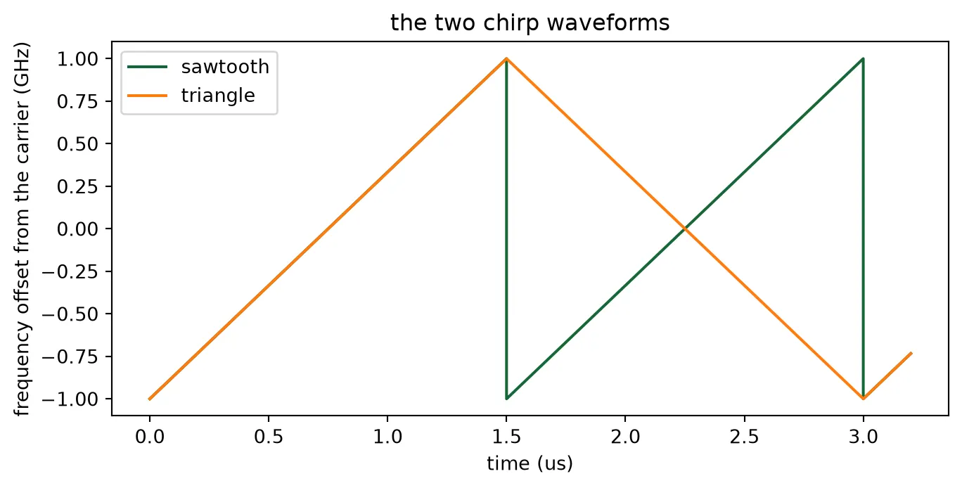

The scene

The scene is the space between the two arrays. The function scene takes the laser field, the heater setting and a list of targets, and returns the fields that enter the chip: the laser at the fibre port and the return at the 32 receive ports. It works in four steps.

Transmit amplitudes. The field at antenna $k$ is the laser field times the chip’s S-matrix amplitude $a_k$ from the fibre to that antenna, times the heater phase $\varphi_k$ of the steering page: $E_k(t) = a_k\, e^{j\varphi_k}\, E(t)$ . The heater phase is applied as a phase rather than as a heater power, because heating a shifter changes an index over a length, and the steering page measured the power that a given phase costs.

Power at the target and back. A target at lateral angle $\psi_t$ and range $R$ is lit with the directivity $G(\psi_t)$ of the steered beam, so a target off the beam axis is lit through the sidelobes. The mean power that its return delivers into the guided modes of the receive antennas is the budget formula with $G(\psi_t)$ in place of the peak directivity.

Delay and Doppler shift. The return is the laser field delayed by the round trip $2R/c$ , rounded to a whole time step, and multiplied by $e^{-2\pi j f_d t}$ with $f_d = 2v/\lambda$ for a target approaching at speed $v$ ; in the envelope convention this raises its frequency.

Distribution over the antennas. The return is a plane wave from $\psi_t$ . Antenna $k$ receives it with the weight $\sqrt{e_k(\psi_t)}$ of its element pattern and the phase $k_0 y_k \sin\psi_t$ of its position, normalized so that the 32 weights carry the power computed above. The two arrays are copies, so by reciprocity the receive array is steered with the same heater phases as the transmit array, and these are applied to the receive fields in the same way.

The function receive then steps the chip. The laser at the fibre port becomes the local oscillator through the tap, the return enters the receive ports, the receive tree combines the 32 fields, the 2x2 coupler mixes the result with the local oscillator, and the two photodiodes convert the two outputs to voltages. The balanced output is the difference of the two. A linear trend is removed from it, which is the DC block of a real receiver: the two photodiodes see slightly different local-oscillator powers, and their difference would otherwise dominate the femtowatt beat. Every call sets up its own time stepper, so each run draws its own shot noise; a reset stepper would replay the same noise. Speckle is not simulated: the scene returns the mean power, and the fade margin remains a budget line.

Reading the beat

The beat frequency is the chirp rate times the round-trip delay,

f_b = \frac{B}{T}\,\frac{2R}{c}, \qquad\text{so}\qquad R = \frac{c\, f_b}{2\,B/T} .

The function spectrum computes the power spectrum of the balanced output with a Hann window and zero padding, and every plot of it uses this relation to label the frequency axis in metres. The function read_range returns the strongest line between 0.5 m, below which the remnant of the DC block sits, and 6 m, the far edge of the scenes on this page. The signal-to-noise ratio of a line is its peak power over the mean noise power per bin, with the line and the skirts of its window excluded from the noise; the factor 1.5 corrects for the noise bandwidth of the Hann window, so the result is the ratio of an unwindowed bin. The amplitude of a beat follows from the peak of its windowed spectrum, $A = 2 |X_\text{peak}| / \sum_n w_n$ , where $w_n$ are the window samples.

def scene(laser, psi_beam, targets):
    """Inputs to the chip for a laser field, a beam steered to psi_beam (deg) and targets given as
    (lateral angle in deg, range in m, reflectivity, speed in m/s toward the chip)."""
    # Heater phases that steer the as-built array to psi_beam, and the antenna amplitudes with them
    phi = heater_phases(psi_beam)
    amps = a_built[i0] * np.exp(1j * phi)
    # Directivity of that beam against the lateral angle
    gain = directivity(amps)
    n_steps = laser.size
    t = np.arange(n_steps) * dt
    rx = np.zeros((n_ch, n_steps), dtype=complex)
    for psi_t, r_t, rho, v in targets:
        # Directivity toward this target
        g_t = np.interp(psi_t, theta, gain)
        # Irradiance at the target per unit laser power: light at the antennas x antenna
        # efficiency x directivity, spread over the sphere of radius r_t
        irradiance = to_antennas * eta_ant * g_t / (4 * np.pi * r_t**2)
        # Radiance of the Lambertian target, and the power its return couples into one mode:
        # radiance x lambda^2 x antenna efficiency x one polarization
        radiance = rho / np.pi * irradiance
        p_return = radiance * (lda0 * 1e-6) ** 2 * eta_ant * polarization
        # Round-trip delay in whole time steps
        m = int(round(2 * r_t / c0 / dt))
        echo = np.zeros(n_steps, dtype=complex)
        echo[m:] = laser[: n_steps - m]
        # Amplitude of the return, and the Doppler shift of an approaching target
        echo *= np.sqrt(p_return) * np.exp(-2j * np.pi * (2 * v / (lda0 * 1e-6)) * t)
        # Weight of each antenna: element pattern toward the target, unit total power
        weights = np.sqrt(
            np.array(
                [np.interp(psi_t, theta, element_by_channel[k]) for k in range(n_ch)]
            )
        )
        weights = weights / np.sqrt(np.sum(weights**2))
        # Phase of the plane wave at each antenna position
        weights = weights * np.exp(1j * k0 * y_ant * np.sin(np.radians(psi_t)))
        rx += np.outer(weights, echo)
    # The laser at the fibre port, and the return at the receive ports with the heater phases
    inputs = {"FIBER@0": laser}
    for k in range(n_ch):
        inputs[f"RX{k}@0"] = rx[k] * np.exp(1j * phi[k])
    return inputs

def receive(inputs):
    """Balanced photodiode voltage of the chip for the given inputs, after the settling time and
    a DC block. Each call sets up its own stepper, so the photodiodes draw fresh shot noise.
    """
    run = pf.CircuitTimeStepper(verbose=False)
    run.setup(chip_feeds, dt, carrier_frequency=f0, show_progress=False)
    out = run.step(pf.TimeSeries(inputs, dt), show_progress=False)
    # Photodiode voltages from the electrical wave amplitudes, and their difference
    v = ((np.real(out["PD_UPPER@0"]) - np.real(out["PD_LOWER@0"])) * np.sqrt(z0))[
        n_settle:
    ]
    # DC block: remove a linear trend
    return v - np.polyval(np.polyfit(np.arange(v.size), v, 1), np.arange(v.size))

def spectrum(v, pad=8, window=True):
    """One-sided power spectrum of a real voltage record, Hann windowed unless told otherwise
    and zero padded by the factor pad, with its frequency axis."""
    w = np.hanning(v.size) if window else np.ones(v.size)
    nfft = pad * v.size
    spec = np.abs(np.fft.rfft(v * w, nfft)) ** 2
    freq = np.fft.rfftfreq(nfft, dt)
    return freq, spec

# Range window searched for a line (m): above the remnant of the DC block, within the scenes
r_min, r_max = 0.5, 6.0

def read_range(freq, spec, chirp_rate=None, r_far=r_max):
    """Beat frequency of the strongest line between r_min and r_far, and the range it
    corresponds to for the given chirp rate (this page's by default)."""
    chirp_rate = slope if chirp_rate is None else chirp_rate
    inside = (freq > 2 * chirp_rate * r_min / c0) & (freq < 2 * chirp_rate * r_far / c0)
    f_b = freq[inside][np.argmax(spec[inside])]
    return f_b, f_b * c0 / (2 * chirp_rate)

def snr(freq, spec, f_b, t_record):
    """Peak power of the line at f_b over the mean noise power per bin. The line and the skirts of
    its window, six bins of the record, are left out of the noise; the factor 1.5 is the noise
    bandwidth of the Hann window."""
    line = np.abs(freq - f_b) < 6 / t_record
    noise = (~line) & (freq > 2 * slope * r_min / c0) & (freq < 500e6)
    return 10 * np.log10(
        spec[np.abs(freq - f_b) < 1 / t_record].max() / np.mean(spec[noise]) * 1.5
    )

def beat_amplitude(v, spec):
    """Amplitude of the strongest beat in a record, from the peak of its Hann-windowed spectrum."""
    return 2 * np.sqrt(spec.max()) / np.hanning(v.size).sum()

One target

The first measurement is a white wall one metre away, on the axis of the broadside beam, with the sawtooth chirp. The chip enters twice: its S matrix sets the transmit amplitudes inside scene, and its time stepper produces the photodiode voltages inside receive. Three numbers are read from the balanced output and compared with the budget.

The range, from the beat frequency and the chirp rate.
The beat amplitude. Each photodiode receives half of the local-oscillator power $P_\text{LO}$ and half of the return $P_\text{rx}$ , and the balanced output is the difference of the two photocurrents times the transimpedance gain, so its amplitude is $2\,\mathcal{R}\,G_\text{TIA}\sqrt{P_\text{LO} P_\text{rx}}$ , with $\mathcal{R}$ the responsivity. $P_\text{LO}$ is the measured steady voltage converted back to power and $P_\text{rx}$ the budget’s returned power after the receive chain.
The signal-to-noise ratio, against the photon count $\eta P_\text{rx} T / h\nu$ for the length of the record.

The photodiode steppers add the shot noise of the light they receive, and the local oscillator dominates it. The return is femtowatts, so the beat is far below the noise in the time trace and is read from the spectrum.

r_wall = 1.0  # Target range (m)

# The sawtooth chirp for one record
laser_cw = pf.abstract.cw_laser(
    power=p_laser, chirp_bandwidth=b_chirp, chirp_period=t_sim
)
source = laser_cw.setup_time_stepper(
    time_step=dt, carrier_frequency=f0, show_progress=False
)
laser = source.step(steps=n_steps, time_step=dt, show_progress=False)["P0@0"]

# The wall on the beam axis, the chip stepped, the spectrum of one clean ramp before the sawtooth wraps
v = receive(scene(laser, 0.0, [(0.0, r_wall, rho_bright, 0.0)]))
window = slice(0, int(round(t_sim / dt)) - n_settle)
freq, spec = spectrum(v[window])
f_b, r_meas = read_range(freq, spec)

# Beat amplitude against the budget: half of the local oscillator and half of the return on each
# photodiode, and the balanced output adds the two beats
p_sig = returned_power(rho_bright, r_wall)
v_beat = 2 * pd_resp * pd_gain * np.sqrt(p_lo_total / 2 * p_sig / 2) * 2
v_meas = beat_amplitude(v[window], spec)
print(
    f"beat {f_b * 1e-6:.2f} MHz -> range {r_meas:.3f} m, set {r_wall:.3f} m ({(r_meas - r_wall) * 100:+.1f} cm; "
    f"a delay step is {c0 * dt / 2 * 100:.2f} cm of range)"
)
print(
    f"beat amplitude {v_meas * 1e3:.2f} mV measured, {v_beat * 1e3:.2f} mV from the budget: "
    f"{20 * np.log10(v_meas / v_beat):+.2f} dB"
)
print(
    f"SNR {snr(freq, spec, f_b, t_sim - t_settle):.1f} dB in a {(t_sim - t_settle) * 1e6:.1f} us record; the budget gives "
    f"{10 * np.log10(quantum_efficiency * p_sig * (t_sim - t_settle) / (h_planck * f0)):.1f} dB for that record"
)

fig, ax = plt.subplots(1, 2, figsize=(12, 4))
t_us = np.arange(v.size) * dt * 1e6
ax[0].plot(t_us[:1000], v[:1000] * 1e3)
ax[0].set_xlabel("time (us)")
ax[0].set_ylabel("balanced output (mV)")
ax[0].set_title("balanced output: local-oscillator shot noise over the beat")
ax[1].plot(freq * c0 / (2 * slope), 10 * np.log10(spec / spec.max()))
ax[1].set_xlim(0, 4)
ax[1].set_ylim(-40, 2)
ax[1].axvline(r_wall, color="gray", linestyle="--", linewidth=1)
ax[1].set_xlabel("range (m)")
ax[1].set_ylabel("beat power (dB)")
ax[1].set_title("range spectrum, white wall at 1 m")
plt.tight_layout()
plt.show()

beat 9.02 MHz -> range 1.014 m, set 1.000 m (+1.4 cm; a delay step is 0.30 cm of range)
beat amplitude 0.91 mV measured, 0.98 mV from the budget: -0.65 dB
SNR 14.9 dB in a 1.4 us record; the budget gives 15.4 dB for that record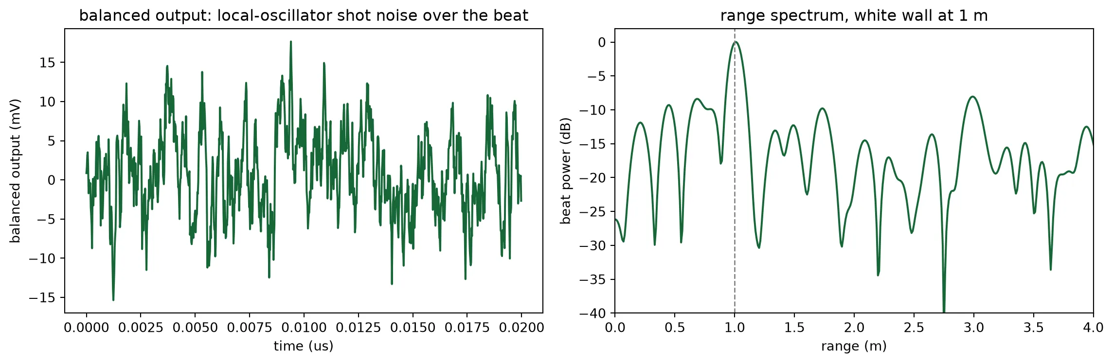

Range and speed from a triangular chirp

An approaching target raises the frequency of the return by the Doppler shift $f_d = 2v/\lambda$ . On the up-ramp this shift subtracts from the range beat, on the down-ramp it adds:

f_\text{up} = f_b - f_d, \qquad f_\text{down} = f_b + f_d .

A triangular chirp therefore gives two beats. Their mean is the range beat and their half difference is the Doppler shift. The target below approaches at 4 m/s from 1.2 m. The record holds one up-ramp and one down-ramp, and each ramp is analysed on its own.

v_target = 4.0  # Approach speed (m/s)
r_moving = 1.2  # Its range (m)

# The triangular chirp: one period holds an up-ramp and a down-ramp of t_sim each
n_tri = 2 * int(round(t_sim / dt)) + n_settle
laser_tri = pf.abstract.cw_laser(
    power=p_laser,
    chirp_bandwidth=b_chirp,
    chirp_period=2 * t_sim,
    chirp_waveform="triangle",
)
source = laser_tri.setup_time_stepper(
    time_step=dt, carrier_frequency=f0, show_progress=False
)
field_tri = source.step(steps=n_tri, time_step=dt, show_progress=False)["P0@0"]

# The moving target, and one spectrum per ramp
v_tri = receive(scene(field_tri, 0.0, [(0.0, r_moving, rho_bright, v_target)]))
n_ramp = int(round(t_sim / dt))
ramps = {
    "up": slice(0, n_ramp - n_settle),
    "down": slice(n_ramp + n_settle, 2 * n_ramp - n_settle),
}
beats = {}
fig, ax = plt.subplots(1, 1, figsize=(8, 4))
for name, sl in ramps.items():
    freq, spec = spectrum(v_tri[sl])
    beats[name], _ = read_range(freq, spec)
    ax.plot(
        freq * 1e-6,
        10 * np.log10(spec / spec.max()),
        label=f"{name} ramp: {beats[name] * 1e-6:.2f} MHz",
    )

# Range from the mean of the two beats, speed from their half difference
f_range = (beats["up"] + beats["down"]) / 2
f_doppler = (beats["down"] - beats["up"]) / 2
print(
    f"range {f_range * c0 / (2 * slope):.3f} m (set {r_moving:.1f} m), speed {f_doppler * lda0 * 1e-6 / 2:.2f} m/s toward the chip (set {v_target:.1f} m/s)"
)
ax.set_xlim(0, 30)
ax.set_ylim(-30, 2)
ax.set_xlabel("beat frequency (MHz)")
ax.set_ylabel("beat power (dB)")
ax.set_title("triangular chirp, target approaching at 4 m/s")
ax.legend()
plt.show()

range 1.198 m (set 1.2 m), speed 4.04 m/s toward the chip (set 4.0 m/s)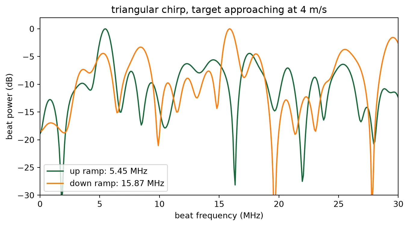

Two targets and the range resolution

Two returns are resolved when their beats differ by one frequency bin of the chirp, $1/T$ . This is a range difference of

\Delta R = \frac{c}{2B} ,

7.5 cm here. Two equal targets 15 cm apart, twice that limit, and 5 cm apart, two thirds of it, show the two sides. The spectra in this cell are taken without the Hann window used elsewhere, because the window widens every line by half a bin. At the limit itself two returns of random relative phase are resolved in some chirps and merge in others.

fig, ax = plt.subplots(1, 2, figsize=(12, 4))
for a, gap in zip(ax, (0.15, 0.05)):
    # Two equal targets on the beam axis, the spectrum without a window and finely padded
    v_two = receive(
        scene(
            laser,
            0.0,
            [(0.0, r_wall, rho_bright, 0.0), (0.0, r_wall + gap, rho_bright, 0.0)],
        )
    )
    freq, spec = spectrum(v_two[window], pad=32, window=False)
    r_axis = freq * c0 / (2 * slope)
    a.plot(r_axis, 10 * np.log10(spec / spec.max()))
    for r in (r_wall, r_wall + gap):
        a.axvline(r, color="gray", linestyle="--", linewidth=1)
    a.set_xlim(r_wall - 0.3, r_wall + gap + 0.3)
    a.set_ylim(-20, 2)
    a.set_xlabel("range (m)")
    a.set_title(
        f"two targets {gap * 100:.0f} cm apart, c / 2B = {c0 / (2 * b_chirp) * 100:.1f} cm"
    )
ax[0].set_ylabel("beat power (dB)")
plt.tight_layout()
plt.show()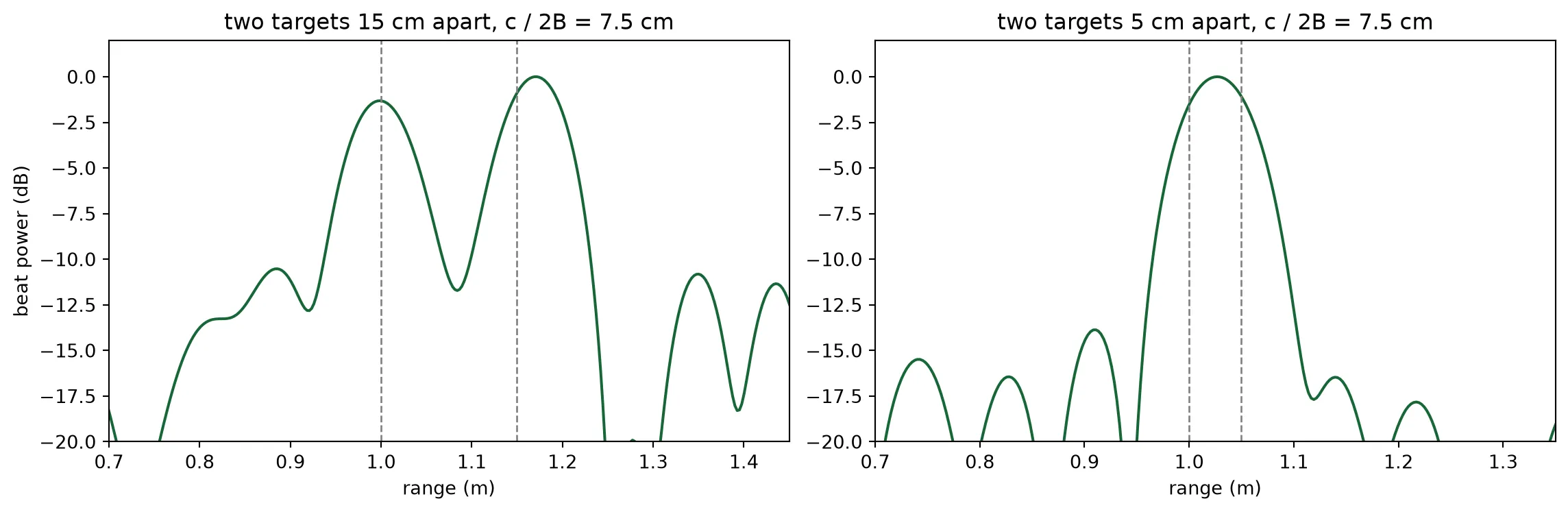

Linewidth and the coherence of the return

The beat is the interference of the return with a copy of the laser delayed by the round trip $\tau$ . Phase noise that accumulates during $\tau$ does not cancel. The phase difference between the two copies has the variance $2\pi\Delta\nu\tau$ , so on average the beat line keeps the fraction

e^{-2\pi\Delta\nu\tau}

of its power, and the rest spreads into a pedestal about $1/\tau$ wide. The coherence time of a Lorentzian line is $1/\pi\Delta\nu$ : 32 ns at 10 MHz, a typical distributed-feedback laser, and 6 ns at 50 MHz, against the 7 ns round trip to the wall. The expected losses are 2 dB at 10 MHz and 9 dB at 50 MHz. A single chirp is one draw of the noise, so a single measurement scatters around these values. The line stands about 16 dB above the shot noise, so the 50 MHz line sits close to the noise floor.

linewidths = (10e6, 50e6)
tau_wall = 2 * r_wall / c0
fig, ax = plt.subplots(1, 1, figsize=(8, 4))
print(
    "linewidth   coherence time   power at the target's beat, against no phase noise   average expected"
)

# The bin of the target's beat in the noise-free spectrum, where the line is read
freq, spec_ref = spectrum(v[window])
f_ref, _ = read_range(freq, spec_ref)
line = np.abs(freq - f_ref) < 1 / (t_sim - t_settle)
for lw in linewidths:
    # The same chirp with phase noise
    laser_lw = pf.abstract.cw_laser(
        power=p_laser, chirp_bandwidth=b_chirp, chirp_period=t_sim, linewidth=lw, seed=3
    )
    source = laser_lw.setup_time_stepper(
        time_step=dt, carrier_frequency=f0, show_progress=False
    )
    field_lw = source.step(steps=n_steps, time_step=dt, show_progress=False)["P0@0"]
    v_lw = receive(scene(field_lw, 0.0, [(0.0, r_wall, rho_bright, 0.0)]))
    freq, spec_lw = spectrum(v_lw[window])
    print(
        f"{lw * 1e-6:6.0f} MHz   {1 / (np.pi * lw) * 1e9:11.0f} ns   {10 * np.log10(spec_lw[line].max() / spec_ref[line].max()):+8.1f} dB"
        f"{10 * np.log10(np.exp(-2 * np.pi * lw * tau_wall)):+38.1f} dB"
    )
    ax.plot(
        freq * 1e-6,
        10 * np.log10(spec_lw / spec_ref.max()),
        label=f"{lw * 1e-6:.0f} MHz linewidth",
    )
ax.plot(
    freq * 1e-6,
    10 * np.log10(spec_ref / spec_ref.max()),
    "k",
    linewidth=0.8,
    label="no phase noise",
)
ax.set_xlim(0, 40)
ax.set_ylim(-30, 2)
ax.set_xlabel("beat frequency (MHz)")
ax.set_ylabel("beat power (dB)")
ax.set_title("beat line against laser linewidth, wall at 1 m")
ax.legend()
plt.show()

linewidth   coherence time   power at the target's beat, against no phase noise   average expected
    10 MHz            32 ns       -0.9 dB                                  -1.8 dB
    50 MHz             6 ns       -3.1 dB                                  -9.1 dB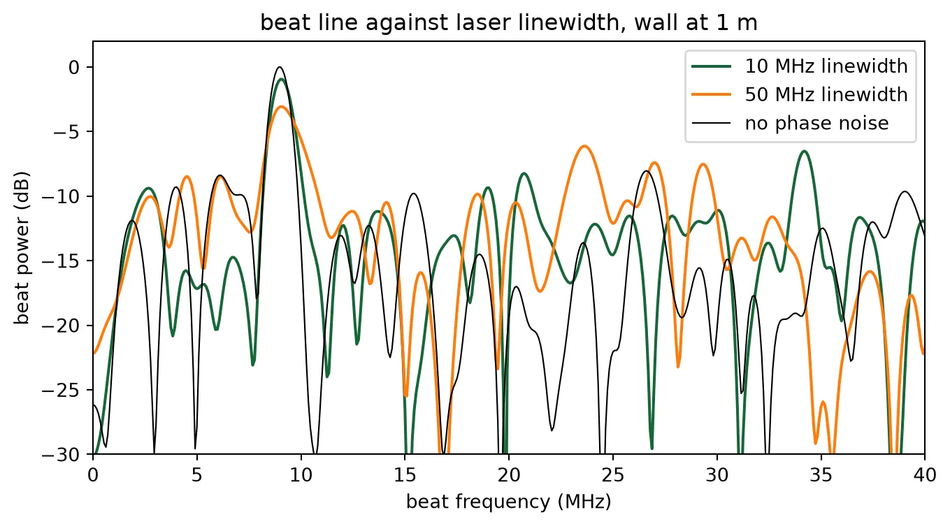

Signal to noise against range

The wall is ranged at three distances. For each, the signal-to-noise ratio is measured at the target’s beat, as the peak power in that bin over the mean noise power per bin, and compared with the budget’s photon count for the same record length. The budget for the 10 us chirp of the system is drawn alongside; it collects seven times the photons of the record stepped here.

test_ranges = (1.0, 2.0, 4.0)
t_record = t_sim - t_settle
measured_snr, budget_snr = [], []
fig, ax = plt.subplots(1, 2, figsize=(12, 4))
for r in test_ranges:
    v_r = receive(scene(laser, 0.0, [(0.0, r, rho_bright, 0.0)]))
    freq, spec_r = spectrum(v_r[window])
    # Read the line at the target's beat, so a line below the noise is reported as such
    near = np.abs(freq - 2 * slope * r / c0) < 2e6
    measured_snr.append(
        snr(freq, spec_r, freq[near][np.argmax(spec_r[near])], t_record)
    )
    # The budget's photon count for this record
    budget_snr.append(
        10
        * np.log10(
            quantum_efficiency
            * returned_power(rho_bright, r)
            * t_record
            / (h_planck * f0)
        )
    )
    print(
        f"wall at {r:3.1f} m: SNR {measured_snr[-1]:5.1f} dB measured at the target's beat, {budget_snr[-1]:5.1f} dB budget"
    )
    ax[0].plot(
        freq * c0 / (2 * slope),
        10 * np.log10(spec_r / spec_r.max()),
        label=f"{r:.1f} m",
    )
ax[0].set_xlim(0, 6)
ax[0].set_ylim(-30, 2)
ax[0].set_xlabel("range (m)")
ax[0].set_ylabel("beat power (dB)")
ax[0].set_title("white wall at three ranges")
ax[0].legend()
ax[1].plot(test_ranges, measured_snr, "o", label="stepped chip")
ax[1].plot(
    ranges,
    10
    * np.log10(
        quantum_efficiency
        * returned_power(rho_bright, ranges)
        * t_record
        / (h_planck * f0)
    ),
    label=f"budget, {t_record * 1e6:.1f} us record",
)
ax[1].plot(
    ranges,
    10
    * np.log10(
        quantum_efficiency
        * returned_power(rho_bright, ranges)
        * t_chirp
        / (h_planck * f0)
    ),
    "--",
    label=f"budget, {t_chirp * 1e6:.0f} us chirp",
)
ax[1].axhline(snr_min, color="gray", linewidth=1)
ax[1].set_xlim(0.5, 20)
ax[1].set_ylim(-10, 30)
ax[1].set_xlabel("range (m)")
ax[1].set_ylabel("SNR (dB)")
ax[1].set_title("signal to noise, white wall")
ax[1].legend()
plt.tight_layout()
plt.show()

wall at 1.0 m: SNR  12.9 dB measured at the target's beat,  15.4 dB budget
wall at 2.0 m: SNR  10.7 dB measured at the target's beat,   9.4 dB budget
wall at 4.0 m: SNR   5.2 dB measured at the target's beat,   3.4 dB budget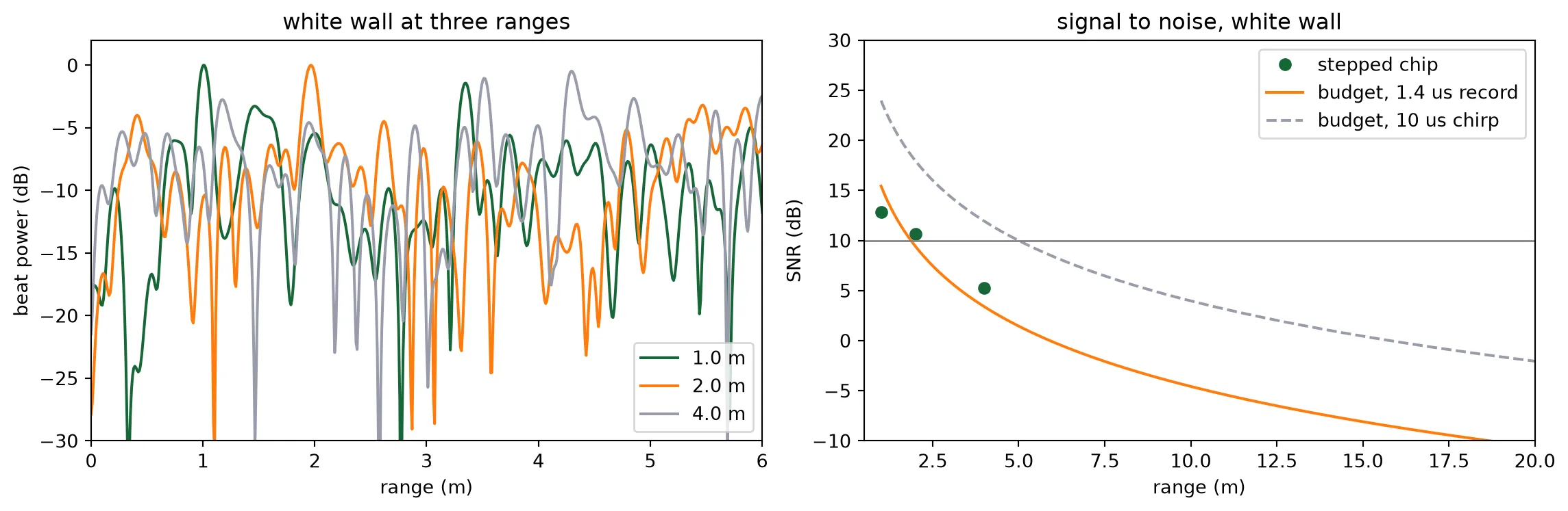

The measured points scatter around the budget’s photon count by a few decibels, which is the spread of a single chirp’s noise, down to the point where the line meets the noise. There the reader returns the noise maximum near the expected beat, so the last point lies above the budget curve rather than on it. The dashed curve is the budget for the 10 us chirp of the system, with the 10 dB threshold five metres out.

A directly modulated laser as the source

The chirp above is an ideal linear sweep. An FMCW source is often a distributed-feedback laser whose current is ramped. The carrier density follows the current, and through the linewidth enhancement factor the frequency follows the carrier density. The library’s directly modulated laser, pf.abstract.dm_laser, solves those rate equations. Its chirp is tied to a power ramp, because the same current sets both, and it exists only above threshold. The cell computes the threshold current from the rate-equation parameters, ramps the current over a range that sweeps about 2 GHz at the same mean power as the fibre laser above, measures the frequency and the power along the ramp, and ranges the same wall with this source.

dml = pf.abstract.dm_laser()
p_dml = dml.active_model.time_stepper.parametric_kwargs

# Threshold current from the rate-equation parameters: the carrier density at which the modal gain
# equals the cavity loss, times the charge that leaves the active region per lifetime
v_g = c0 / p_dml["n_group"]
n_th = p_dml["transparency_carrier_density"] + 1 / (
    p_dml["confinement_factor"]
    * v_g
    * p_dml["differential_gain"]
    * p_dml["photon_lifetime"]
)
i_th = q_e * p_dml["active_region_volume"] * n_th / p_dml["carrier_lifetime"]
# A ramp that sweeps about 2 GHz at the fibre laser's mean power
i_low, i_high = 2.0 * i_th, 3.0 * i_th
print(
    f"threshold {i_th * 1e3:.1f} mA; ramp {i_low * 1e3:.1f} to {i_high * 1e3:.1f} mA over {t_sim * 1e6:.1f} us"
)

# Settle at the low current, then ramp; the current enters the electrical port as a wave amplitude
n_pre = int(round(200e-9 / dt))
current = np.concatenate([np.full(n_pre, i_low), np.linspace(i_low, i_high, n_steps)])
dml_stepper = dml.setup_time_stepper(
    time_step=dt, carrier_frequency=f0, show_progress=False
)
laser_dml = dml_stepper.step(
    pf.TimeSeries({"E0@0": current * np.sqrt(z0)}, dt), show_progress=False
)["P0@0"][n_pre:]

# The chirp rate of this source, from a straight-line fit to its instantaneous frequency
freq_dml = instantaneous_frequency(laser_dml)
fit = np.polyfit(t[n_settle:], freq_dml[n_settle:], 1)
slope_dml = fit[0]
print(
    f"sweep {(freq_dml[-1] - freq_dml[n_settle]) * 1e-9:.2f} GHz at {slope_dml * 1e-12:.0f} MHz per us, "
    f"deviation from a straight line {np.std(freq_dml[n_settle:] - np.polyval(fit, t[n_settle:])) * 1e-6:.1f} MHz rms; "
    f"power {np.abs(laser_dml[n_settle]) ** 2 * 1e3:.1f} to {np.abs(laser_dml[-1]) ** 2 * 1e3:.1f} mW"
)

# The wall ranged with this source; the range axis uses its own chirp rate
v_dml = receive(scene(laser_dml, 0.0, [(0.0, r_wall, rho_bright, 0.0)]))
freq, spec_dml = spectrum(v_dml[window])
f_b, r_dml = read_range(freq, spec_dml, chirp_rate=slope_dml)
print(f"range {r_dml:.3f} m read with the DM laser (set {r_wall:.1f} m)")

fig, ax = plt.subplots(1, 3, figsize=(15, 4))
ax[0].plot(t * 1e6, freq_dml * 1e-9)
ax[0].set_xlabel("time (us)")
ax[0].set_ylabel("frequency offset (GHz)")
ax[0].set_title("chirp of the DM laser under the current ramp")
ax[1].plot(t * 1e6, np.abs(laser_dml) ** 2 * 1e3)
ax[1].set_xlabel("time (us)")
ax[1].set_ylabel("power (mW)")
ax[1].set_title("its power over the ramp")
ax[2].plot(
    freq * c0 / (2 * slope_dml),
    10 * np.log10(spec_dml / spec_dml.max()),
    label="DM laser",
)
ax[2].plot(
    freq * c0 / (2 * slope),
    10 * np.log10(spec_ref / spec_ref.max()),
    "k",
    linewidth=0.8,
    label="ideal chirp",
)
ax[2].set_xlim(0, 3)
ax[2].set_ylim(-30, 2)
ax[2].set_xlabel("range (m)")
ax[2].set_ylabel("beat power (dB)")
ax[2].set_title("range spectrum with each source")
ax[2].legend()
plt.tight_layout()
plt.show()

threshold 35.9 mA; ramp 71.7 to 107.6 mA over 1.5 us
sweep 2.22 GHz at 1479 MHz per us, deviation from a straight line 0.1 MHz rms; power 6.1 to 11.4 mW
range 1.014 m read with the DM laser (set 1.0 m)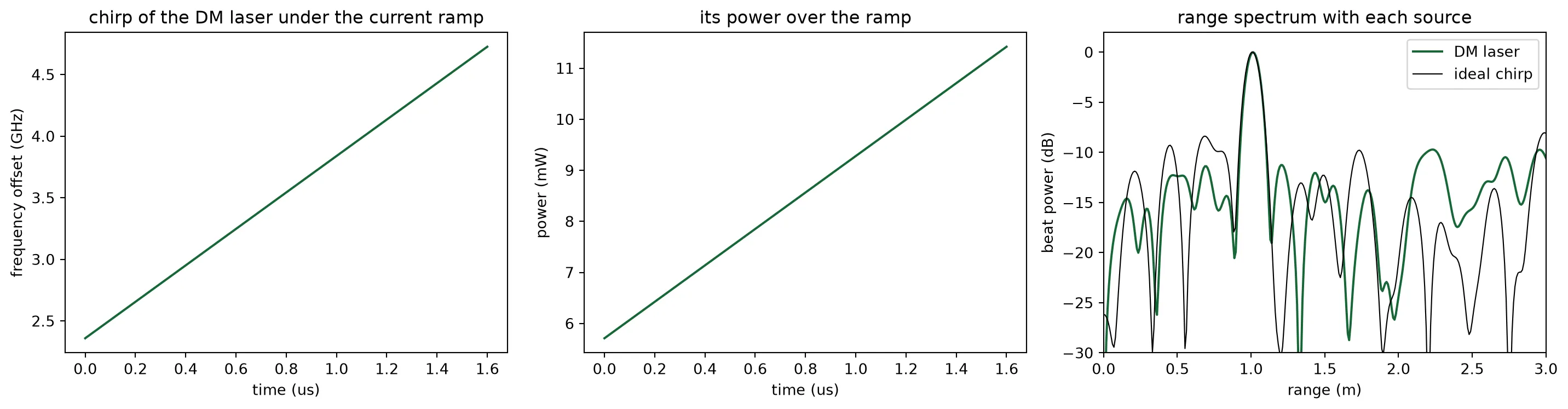

The rate equations give an almost linear sweep, since the frequency follows the carrier density and the carrier density follows the current. The 2 GHz excursion costs a ramp of a few tens of milliamperes, over which the power nearly doubles. This amplitude modulation is what the model adds: the beat amplitude ramps with the power, and the range peak stays where the ideal chirp puts it. A real device adds the thermal and nonlinear chirp that the rate equations leave out, which is what commercial systems linearize against.

The scene image

The last measurement uses the steering. The beam is set to five lateral angles with the heater phases of the steering page. Six targets stand at different angles and ranges, one of them between two beam positions. Each beam setting gives one range spectrum. Stacked side by side, the five spectra form the range image of the scene along one axis: range against lateral angle. The sidelobes and the beam width decide how much of each target leaks into the neighbouring columns. The strongest line of each column is read within the 3 m window of the image.

beam_angles = (-20.0, -10.0, 0.0, 10.0, 20.0)
targets = [
    (-20.0, 1.0, rho_bright, 0.0),
    (-10.0, 1.2, rho_bright, 0.0),
    (0.0, 1.3, rho_bright, 0.0),
    (5.0, 1.3, rho_bright, 0.0),
    (10.0, 0.8, rho_bright, 0.0),
    (20.0, 1.45, rho_bright, 0.0),
]
image = []
for psi_b in beam_angles:
    # All six targets seen by the beam at psi_b, one spectrum per beam setting
    v_b = receive(scene(laser, psi_b, targets))
    freq, spec_b = spectrum(v_b[window])
    image.append(spec_b)
    # The strongest line within the 3 m window of the image
    f_b, r_b = read_range(freq, spec_b, r_far=3.0)
    print(f"beam at {psi_b:+5.1f} deg: strongest return at {r_b:.2f} m")
image = np.array(image)
r_axis = freq * c0 / (2 * slope)
keep = r_axis < 3.0

fig, ax = plt.subplots(1, 1, figsize=(8, 5))
pcm = ax.pcolormesh(
    beam_angles,
    r_axis[keep],
    10 * np.log10(image[:, keep].T / image.max()),
    vmin=-25,
    vmax=0,
    cmap="magma",
    shading="nearest",
)
for psi_t, r_t, _, _ in targets:
    ax.plot(psi_t, r_t, "wo", markerfacecolor="none", markersize=9)
ax.set_xlabel("beam angle, lateral (deg)")
ax.set_ylabel("range (m)")
ax.set_title("range image of the scene; circles mark the targets")
plt.colorbar(pcm, ax=ax, label="beat power (dB)")
plt.show()

beam at -20.0 deg: strongest return at 1.00 m
beam at -10.0 deg: strongest return at 1.19 m
beam at  +0.0 deg: strongest return at 1.32 m
beam at +10.0 deg: strongest return at 0.80 m
beam at +20.0 deg: strongest return at 1.47 m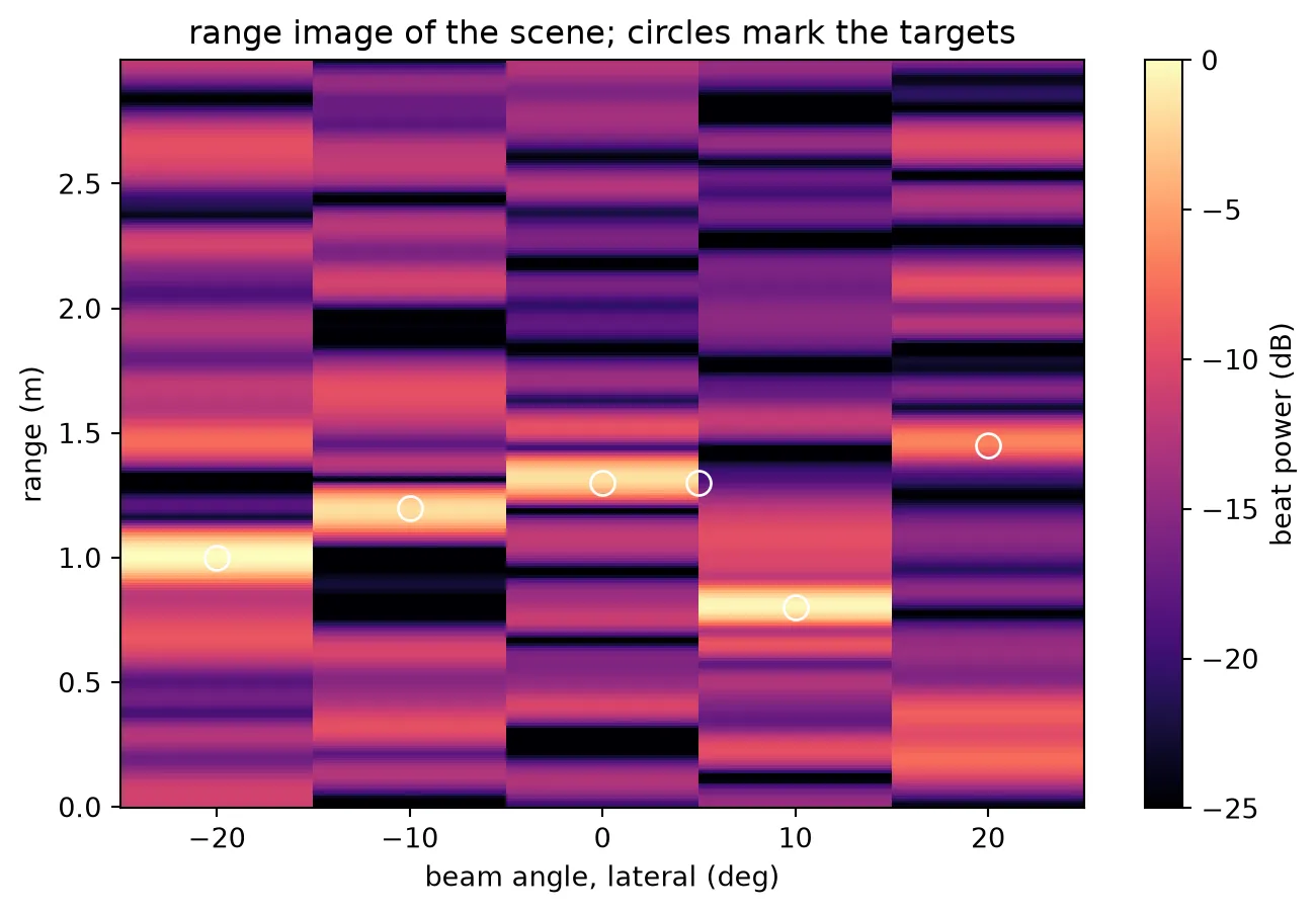

Every target on a beam axis appears in its column at its range. The target at 5 degrees sits between two beam positions and appears in both neighbouring columns, weaker in each. This is how a phased-array LiDAR sees between its resolvable positions: the two-degree beam width and the ten-degree step between the settings decide how much of it each column catches. Returns from the targets of the other columns leak in through the sidelobes at the level the steering page measured.

Summary of the series

Six pages took the LiDAR from a requirement, ten metres of range and 7.5 cm of resolution, to a beat on the two photodiodes of a drawn and verified chip. The technology page turned the requirement into an aperture and a stack. The antenna page designed the grating antenna step by step, and found that the pitch had to drop below the wavelength and that the emission angle does not change the radiated power. The component page attached a measured model to every other cell. The layout page drew the chip and verified its wiring. The steering page pointed the beam and computed the heater power. This page assembled the budget from all those measurements and compared it with the stepped chip: the beat amplitude and the signal-to-noise ratio agree with the budget within the spread of a single chirp’s shot noise. A 10 mW laser through this aperture ranges a white wall at five metres and a dark target at two, and speckle decides how reliably.