LiDAR Component Library

Download notebook (.zip)

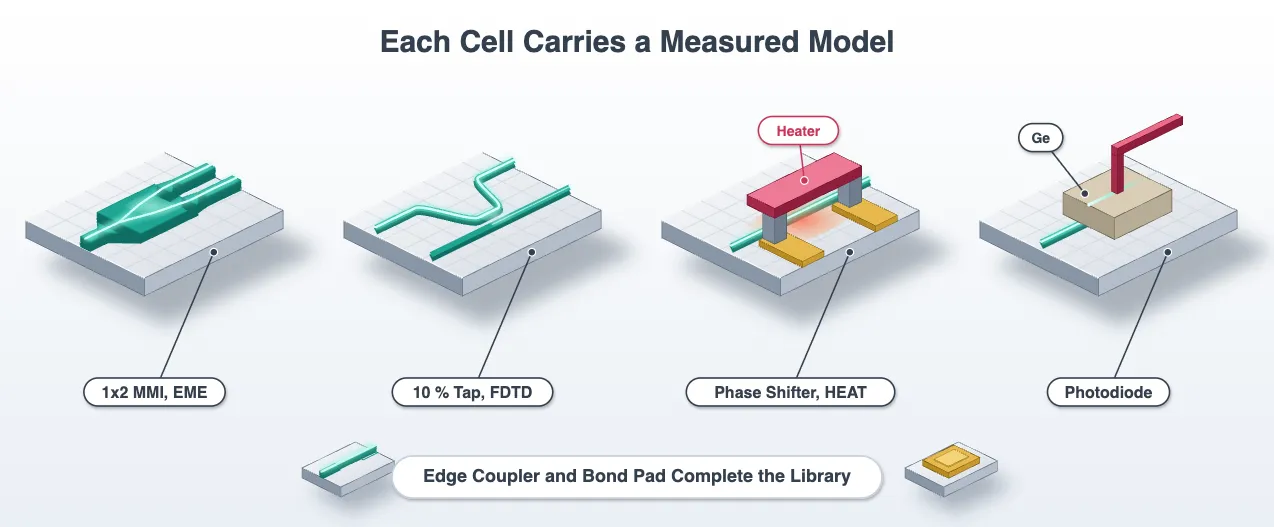
This notebook turns the process stack from LiDAR System Budget and Technology into devices. The chip needs nine: two grating antennas, one for each strip width, a 1x2 splitter, a 2x2 coupler for the coherent mixer, a local-oscillator tap, a thermo-optic phase shifter, a germanium photodiode, an edge coupler and a bond pad.

The antenna has its own page, the grating antenna design, because every one of its numbers has to be measured. This page takes its two antenna cells and their measured numbers as given. The splitters are designed by an EME length sweep and the tap by a short FDTD sweep. The phase shifter gets an analytic model with one unknown, the temperature rise per milliwatt, which the beam steering page measures with a heat solve.

# The technology, the media, the wavelength grid and the grating indices come from
from runpy import run_path

# Lidar_Antenna.qmd defines what this notebook builds on. Its shared cells are
# generated into the module below; see docs/scripts/generate_notebook_modules.py.
globals().update(
    {k: v for k, v in run_path("misc/lidar_antenna.py").items() if not k.startswith("_")}
)

import photonforge.abstract as pfa
from photonforge.live_viewer import LiveViewer
from photonforge.utils import virtual_port_spec

viewer = LiveViewer()

# Read the widths off the technology rather than repeating them, so changing
# them in Lidar_Technology.qmd changes them here too
w_core = tech.parametric_kwargs["core_width"]

# Sidewall scattering, which no mode solve predicts, so it comes from process
# data. Two dB/cm suits a strip waveguide; substitute the fab's own figure.
scattering_db_cm = 2.0

# Width of every drawn metal trace and terminal. A property of the layer rather
# than of any one device, so the cells below read it from here.
metal_width = 3.0

# Index of the design frequency in the shared wavelength grid
i0 = int(np.argmin(np.abs(freqs - f0)))

LiveViewer started at http://127.0.0.1:33709. Call its 'stop()' method to free the port.

The splitters

A multimode interferometer (MMI) splits light by self-imaging: a wide section supports several modes that beat against each other and reproduce the input field, in one or more copies, at fixed distances. With the input on the axis of a section of width $W$ , two images appear at $L = 3 L_\pi / 8$ , where $L_\pi$ is the beat length of the two lowest modes; with the input off axis, two images appear at $3 L_\pi / 2$ . The first makes the 1x2 splitter that fans the laser out to 32 antennas, the second the 2x2 coupler that mixes the return with the local oscillator.

Both are the same cell with a different port count, so one parametric component covers them. The access waveguides taper from 500 nm to 1.5 um at the wide section, which excites fewer unwanted modes and lowers the excess loss. The model is EMEModel: eigenmode expansion solves the modes of each cross-section once and propagates them analytically, which suits a device that is a few uniform sections in series. The wide section is one EME cell, since propagation in a uniform section is exact, and each taper gets eight.

@pf.parametric_component(name_prefix="MMI")
def mmi(
    *,
    num_ports=(1, 2),
    length=15.0,
    mmi_width=4.0,
    port_length=5.0,
    taper_width=1.5,
    port_separation=2.0,
    num_modes=20,
    taper_cells=8
):
    c = pf.Component()
    port_spec = pf.config.default_technology.ports["TE_1550_500"]

    # Wide section, linear tapers and access waveguides in one stencil
    c.add(
        "Si",
        *pf.stencil.mmi(
            length=length,
            width=mmi_width,
            num_ports=num_ports,
            port_length=port_length,
            port_width=w_core,
            tapered_width=taper_width,
            port_separation=port_separation,
        )
    )
    c.add_port(c.detect_ports([port_spec]))

    # EME cells: taper_cells per taper, a single cell for the uniform wide section
    x_min = c.bounds()[0][0]
    mode_spec = td.EMEModeSpec(num_modes=num_modes)
    eme_grid = td.EMECompositeGrid(
        subgrids=[
            td.EMEUniformGrid(num_cells=taper_cells, mode_spec=mode_spec),
            td.EMEUniformGrid(num_cells=1, mode_spec=mode_spec),
            td.EMEUniformGrid(num_cells=taper_cells, mode_spec=mode_spec),
        ],
        subgrid_boundaries=[x_min + port_length, x_min + port_length + length],
    )
    # The EME window across the device follows the port windows by default, which would
    # put the boundary on the wide section's sidewall; widen it to leave cladding outside
    half_window = mmi_width / 2 + 2.0
    c.add_model(
        pf.EMEModel(
            eme_grid_spec=eme_grid,
            bounds=((None, -half_window, None), (None, half_window, None)),
            verbose=False,
        ),
        "EME",
    )
    return c

splitter = mmi(num_ports=(1, 2))
print("1x2 ports:", list(splitter.ports))
viewer(splitter)

1x2 ports: ['P0', 'P1', 'P2']

Finding the image lengths

The beat length from the slab index of a 4 um section puts the two-fold images near 15 um for the 1x2 and 58 um for the 2x2, but the tapers and the finite width move them, so each length is swept.

The sweep does not rebuild the device at every length. The wide section is a single EME cell, and a tidy3d.EMELengthSweep passed through the model’s simulation_updates rescales that one cell: the modes are solved once and only the analytic propagation through the section changes, so a sweep of sixty lengths is one simulation. The scale_factors array has one row per length and one column per EME cell, all ones except the column of the wide section. The sweep returns the S matrix in the basis of the facet modes, and a facet with two waveguides has an even and an odd supermode, so the power in each waveguide is the power in their sum and difference.

For both cells the image length is where the most power reaches the outputs, because that is where the images are sharpest. The 1x2 is balanced by symmetry; the balance of the 2x2 at its image length is something to check, and it is checked across the band below.

sweeps = {
    (1, 2): dict(base=16.0, lengths=np.linspace(8.0, 24.0, 65)),
    (2, 2): dict(base=57.0, lengths=np.linspace(46.0, 68.0, 56)),
}

# One base cell per device, and a separate model carrying the length sweep, so the cell's
# own model stays untouched for the spectra later
for ports, sw in sweeps.items():
    cell = mmi(num_ports=ports, length=sw["base"])
    model = cell.models["EME"]
    num_cells = sum(sub.num_cells for sub in model.eme_grid_spec.subgrids)

    # Scale only the wide-section cell, which follows the input taper's cells
    scale = np.ones((sw["lengths"].size, num_cells))
    scale[:, cell.parametric_kwargs["taper_cells"]] = sw["lengths"] / sw["base"]
    sw["cell"] = cell
    sw["model"] = pf.EMEModel(
        eme_grid_spec=model.eme_grid_spec,
        bounds=model.bounds,
        verbose=False,
        simulation_updates={
            "sweep_spec": td.EMELengthSweep(scale_factors=scale.tolist())
        },
    )
    # Submit both sweeps before reading either
    sw["model"].start(cell, [f0])

# S matrix from the input facet to the output facet, indexed (length, output mode, input mode)
for ports, sw in sweeps.items():
    sw["s"] = (
        sw["model"]
        .simulation_data(sw["cell"], [f0], show_progress=False)
        .smatrix.S21.isel(f=0)
        .values
    )

# 1x2: one input mode; the two output waveguides carry the sum and difference of the
# even and odd facet modes, and the total is what the image length maximizes
s = sweeps[(1, 2)]["s"]
even, odd = s[:, 0, 0], s[:, 1, 0]
out_12 = np.stack([np.abs(even + odd) ** 2 / 2, np.abs(even - odd) ** 2 / 2], axis=1)
total_12 = out_12.sum(axis=1)

# 2x2: light in one input waveguide is the sum of the two input facet modes, and the same
# projection gives the two outputs. The spectra below name bar and cross from the port basis.
s = sweeps[(2, 2)]["s"]
even_out = (s[:, 0, 0] + s[:, 0, 1]) / np.sqrt(2)
odd_out = (s[:, 1, 0] + s[:, 1, 1]) / np.sqrt(2)
out_22 = np.stack(
    [np.abs(even_out + odd_out) ** 2 / 2, np.abs(even_out - odd_out) ** 2 / 2], axis=1
)
total_22 = out_22.sum(axis=1)

# Image lengths: where the most power reaches the outputs
lengths_12, lengths_22 = sweeps[(1, 2)]["lengths"], sweeps[(2, 2)]["lengths"]
length_12 = float(lengths_12[np.argmax(total_12)])
length_22 = float(lengths_22[np.argmax(total_22)])
print(f"1x2 image length {length_12:.2f} um, 2x2 image length {length_22:.1f} um")
print(
    f"at the 2x2 image the two outputs carry {10 * np.log10(out_22[np.argmax(total_22)]).round(2)} dB"
)
print(
    f"excess loss at the image: 1x2 splitter {-10 * np.log10(total_12.max()):.2f} dB, "
    f"2x2 coupler {-10 * np.log10(total_22.max()):.2f} dB"
)

fig, ax = plt.subplots(1, 2, figsize=(11, 4))
ax[0].plot(lengths_12, 10 * np.log10(total_12))
ax[0].axvline(length_12, color="gray", linestyle="--", linewidth=1)
ax[0].set_xlabel("wide section length (um)")
ax[0].set_ylabel("power to both outputs (dB)")
ax[0].set_title("1x2 splitter")
ax[1].plot(lengths_22, 10 * np.log10(out_22[:, 0]), label="one output")
ax[1].plot(lengths_22, 10 * np.log10(out_22[:, 1]), label="other output")
ax[1].plot(lengths_22, 10 * np.log10(total_22), color="gray", label="both")
ax[1].axvline(length_22, color="gray", linestyle="--", linewidth=1)
ax[1].set_xlabel("wide section length (um)")
ax[1].set_ylabel("power (dB)")
ax[1].set_title("2x2 coupler")
ax[1].legend()
plt.tight_layout()
plt.show()

1x2 image length 14.00 um, 2x2 image length 56.8 um
at the 2x2 image the two outputs carry [-3.1 -3.2] dB
excess loss at the image: 1x2 splitter 0.05 dB, 2x2 coupler 0.15 dB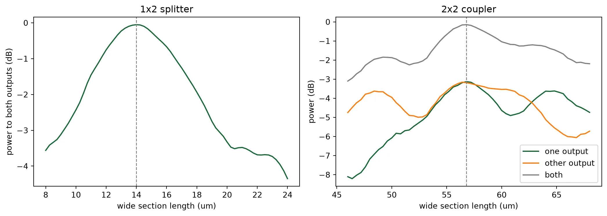

The splitters across the band

The two cells are rebuilt at their image lengths and solved across the tuning range. The 1x2 has to stay balanced, which symmetry guarantees, and low loss. The 2x2 has to stay at 3 dB, which nothing guarantees, and it has to put its two outputs 90 degrees apart, because the balanced receiver subtracts the two photocurrents and that phase is what makes the local-oscillator terms cancel while the beat terms add.

splitter = mmi(num_ports=(1, 2), length=length_12)
mixer = mmi(num_ports=(2, 2), length=length_22)

# Both spectra submitted before either is read
for cell in (splitter, mixer):
    cell.models["EME"].start(cell, freqs, inputs=["P0"])
s_split = splitter.s_matrix(freqs, model_kwargs={"inputs": ["P0"]}, show_progress=False)
s_mix = mixer.s_matrix(freqs, model_kwargs={"inputs": ["P0"]}, show_progress=False)

# Output powers in dB, and the bar-cross phase of the 2x2
split_out = 10 * np.log10(np.abs(s_split[("P0@0", "P1@0")]) ** 2)
mix_bar = 10 * np.log10(np.abs(s_mix[("P0@0", "P2@0")]) ** 2)
mix_cross = 10 * np.log10(np.abs(s_mix[("P0@0", "P3@0")]) ** 2)
mix_phase = np.degrees(np.angle(s_mix[("P0@0", "P3@0")] / s_mix[("P0@0", "P2@0")]))

print(
    f"1x2: {split_out[i0]:.2f} dB per output at 1550 nm, excess loss {-(split_out[i0] + 3.01):.2f} dB"
)
print(
    f"2x2: bar {mix_bar[i0]:.2f} dB, cross {mix_cross[i0]:.2f} dB, "
    f"phase {mix_phase[i0]:.0f} deg at 1550 nm"
)

fig, ax = plt.subplots(1, 2, figsize=(11, 4))
ax[0].plot(wavelengths * 1e3, split_out, label="1x2, each output")
ax[0].plot(wavelengths * 1e3, mix_bar, label="2x2, bar")
ax[0].plot(wavelengths * 1e3, mix_cross, label="2x2, cross")
ax[0].axhline(-3.01, color="gray", linestyle="--", linewidth=1)
ax[0].set_xlabel("wavelength (nm)")
ax[0].set_ylabel("transmission (dB)")
ax[0].set_title("splitting across the band")
ax[0].legend()
ax[1].plot(wavelengths * 1e3, mix_phase)
ax[1].set_xlabel("wavelength (nm)")
ax[1].set_ylabel("cross minus bar phase (deg)")
ax[1].set_title("2x2 output phase")
plt.tight_layout()
plt.show()

1x2: -3.07 dB per output at 1550 nm, excess loss 0.06 dB
2x2: bar -3.13 dB, cross -3.19 dB, phase -91 deg at 1550 nm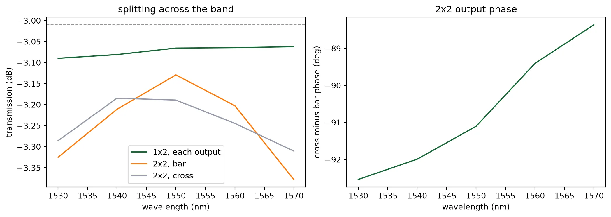

The 1x2 loses under a tenth of a decibel over the band. The 2x2 stays within a few hundredths of a decibel of 3 dB and its outputs within a few degrees of quadrature, which is what the balanced receiver needs: the local-oscillator power appears equally on both photodiodes and cancels in their difference, while the beat terms arrive in antiphase and add.

The local-oscillator tap

The receiver needs a copy of the transmitted light to beat the return against. Ten percent of the laser is taken off before the splitter tree by a directional coupler: two strip waveguides brought to a 200 nm gap by S bends, with a straight coupling section whose length sets the fraction. The coupled power follows $\sin^2(\kappa_0 + \kappa' L)$ , where $\kappa_0$ is what the S bends alone couple and $\kappa'$ the coupling per unit length, so three FDTD runs at three lengths fix both and the length for ten percent follows.

tap_gap = 0.2  # Gap of the coupling section (um)
tap_lengths = (0.0, 3.0, 6.0)

def tap_at(coupling_length):
    return pf.parametric.s_bend_straight_coupler(
        port_spec="TE_1550_500",
        coupling_distance=w_core + tap_gap,
        s_bend_length=12.0,
        s_bend_offset=6.0,  # enough offset to clear the bus for the route to the mixer
        coupling_length=coupling_length,
        euler_fraction=0.5,
        model=pf.Tidy3DModel(grid_spec=14, verbose=False),
    )

# Submit the three lengths together, then read the coupled fraction of each;
# P0 and P2 are the bus, P3 is the tap
taps = [tap_at(length) for length in tap_lengths]
for cell in taps:
    cell.active_model.start(cell, [f0], inputs=["P0"])
coupled = []
for cell in taps:
    s = cell.s_matrix([f0], model_kwargs={"inputs": ["P0"]}, show_progress=False)
    coupled.append(abs(s[("P0@0", "P3@0")][0]) ** 2)
coupled = np.array(coupled)

# sin^2 law: the arcsine of the amplitude is linear in length
kappa_fit = np.polyfit(tap_lengths, np.arcsin(np.sqrt(coupled)), 1)
tap_fraction = 0.1  # Fraction of the laser sent to the local oscillator
tap_length = float((np.arcsin(np.sqrt(tap_fraction)) - kappa_fit[1]) / kappa_fit[0])
for length, frac in zip(tap_lengths, coupled):
    print(f"coupling length {length:.0f} um: {frac * 100:.1f} percent")
print(
    f"\n{kappa_fit[0]:.4f} rad/um from the straight section, {np.degrees(kappa_fit[1]):.1f} deg from the S bends"
)
print(f"coupling length for {tap_fraction * 100:.0f} percent: {tap_length:.2f} um")

coupling length 0 um: 2.6 percent
coupling length 3 um: 8.3 percent
coupling length 6 um: 17.0 percent

0.0440 rad/um from the straight section, 9.2 deg from the S bends
coupling length for 10 percent: 3.66 um

The tap is rebuilt at that length and simulated once more to read its four coefficients. Those then replace the FDTD model with a DirectionalCouplerModel, so the chip pages do not re-solve a coupler each time they ask for an S matrix. The coupled amplitude is rotated into quadrature with the transmitted one before it is handed over. A lossless four-port has its two outputs 90 degrees apart, and the measured pair are not, because the tap arm leaves on an S bend and is longer than the straight bus. Handing the model the raw pair makes it non-passive by a few percent, which a time-domain fit turns into a fraction of a decibel of error. The Optical I/O component library works through the same rotation for its monitor tap.

tap = tap_at(tap_length)
s_tap = tap.s_matrix([f0], model_kwargs={"inputs": ["P0"]}, show_progress=False)
coef = {k: complex(s_tap[("P0@0", f"{k}@0")][0]) for k in ("P0", "P1", "P2", "P3")}

print(f"tapped      {abs(coef['P3'])**2 * 100:.1f} percent")
print(f"bus loss    {-10 * np.log10(abs(coef['P2'])**2):.3f} dB")
print(f"isolation   {abs(coef['P1'])**2:.1e}")
print(f"reflection  {abs(coef['P0'])**2:.1e}")

# Rotate the coupled amplitude into quadrature with the transmitted one
c_quad = abs(coef["P3"]) * coef["P2"] / abs(coef["P2"]) * -1j

# Replace FDTD with the numbers it just produced
tap.add_model(
    pf.DirectionalCouplerModel(
        t=coef["P2"], c=c_quad, i=0, r=0, ports=["P0", "P1", "P2", "P3"]
    ),
    "compact",
)
print(f"active model now {tap.active_model_name}")
viewer(tap)

tapped      10.0 percent
bus loss    0.460 dB
isolation   7.4e-06
reflection  1.0e-06
active model now compact

The thermo-optic phase shifter

Each antenna gets a phase shifter: a straight strip waveguide with the TiN heater above it and a via to an M1 feed at each end, as drawn on the technology page. Heat raises the silicon index by $dn/dT \approx 1.8 \times 10^{-4}$ per kelvin, and a temperature rise $\Delta T$ over a length $L$ shifts the phase by $2\pi\, (dn_\text{eff}/dT)\, \Delta T\, L / \lambda$ . A π shift needs

\Delta T_\pi = \frac{\lambda}{2 L\, dn_\text{eff}/dT},

which is about 20 K for a 200 um heater. The power that buys it depends on the thermal impedance of the heater, in kelvin per milliwatt, and that impedance falls as the heater gets longer, so for a straight heater $P_\pi$ hardly depends on length: a longer heater needs fewer kelvin and gets fewer kelvin per milliwatt in the same proportion. Length is chosen for the resistance, since the drive voltage is $\sqrt{P R}$ , and for footprint. The impedance is the one number this cell does not supply. It comes from a heat solve of the cross-section on the beam steering page, which gives 1.08 K per milliwatt for this heater. That value is entered here so that the model is complete.

The model is an AnalyticWaveguideModel carrying the strip index, the group index, the scattering loss and the thermo-optic coefficient, evaluated at the heated temperature. Its time stepper is set to the analytic waveguide stepper rather than the default pole fit, because a length of waveguide is a pure delay and the fit cannot hold one reliably.

dn_dt = 1.8e-4  # Thermo-optic coefficient of the strip mode (1/K)
# Thermal impedance from the heat solve on the steering page (K/mW)
k_thermal_measured = 1.08
# Electrical conductivity of the heater film (S/um), from the technology
tin_conductivity = 2.3
t_ambient = 293.0  # Reference temperature of the model (K)

@pf.parametric_component(name_prefix="PS")
def phase_shifter(
    *,
    length=200.0,
    heater_width=1.0,
    via_length=3.0,
    power=0.0,
    k_thermal=k_thermal_measured,
):
    c = pf.Component()
    port_spec = pf.config.default_technology.ports["TE_1550_500"]

    # Strip core along x with the heater strip centred above it
    c.add(
        "Si",
        pf.Rectangle((0, -w_core / 2), (length, w_core / 2)),
        "Heater",
        pf.Rectangle((0, -heater_width / 2), (length, heater_width / 2)),
    )

    # A via on each heater end, and an M1 terminal on top of it for the chip to route from
    for name, x_end, sign in (("H0", 0.0, 1), ("H1", length, -1)):
        landing = pf.Rectangle((x_end, -0.4), (x_end + sign * via_length, 0.4))
        c.add("Via", landing)
        c.add_terminal(
            pf.Terminal(
                "M1",
                pf.Rectangle(
                    center=(x_end + sign * via_length / 2, 0),
                    size=(metal_width, metal_width),
                ),
            ),
            name,
            add_structure=True,
        )

    # Both ends are plain strip, so the ports are found from the geometry
    c.add_port(c.detect_ports([port_spec]))

    # Temperature rise from the electrical power through the thermal impedance
    delta_t = k_thermal * power

    # Analytic waveguide at the heated temperature, with its delay-holding stepper
    model = pf.AnalyticWaveguideModel(
        n_eff=n_eff_strip,
        n_group=n_group_strip,
        propagation_loss=scattering_db_cm * 1e-4,  # dB/cm to dB/um
        dn_dT=dn_dt,
        temperature=t_ambient + delta_t,
        reference_temperature=t_ambient,
        reference_frequency=f0,
    )
    model.time_stepper = pf.AnalyticWaveguideTimeStepper(
        n_eff=n_eff_strip + dn_dt * delta_t,
        n_group=n_group_strip,
        propagation_loss=scattering_db_cm * 1e-4,
    )
    c.add_model(model, "thermal")
    return c

ps = phase_shifter()
l_heater = ps.parametric_kwargs["length"]
w_heater = ps.parametric_kwargs["heater_width"]

# Heater resistance from the film conductivity and its cross-section
r_heater = l_heater / (
    tin_conductivity * w_heater * tech.parametric_kwargs["heater_thickness"]
)

# Power and voltage for a pi shift
dt_pi = lda0 / (2 * l_heater * dn_dt)
p_pi = dt_pi / k_thermal_measured
print(f"heater {l_heater:.0f} um x {w_heater:.1f} um: {r_heater:.0f} ohm")
print(
    f"pi shift needs {dt_pi:.1f} K, about {p_pi:.0f} mW and {np.sqrt(p_pi * 1e-3 * r_heater):.1f} V "
    f"at {k_thermal_measured} K/mW"
)
viewer(ps)

heater 200 um x 1.0 um: 725 ohm
pi shift needs 21.5 K, about 20 mW and 3.8 V at 1.08 K/mW

The phase against power is read off the model itself, by rebuilding the cell at a set of drive powers and taking the transmission phase at the design wavelength. It is a straight line, since the model is linear in temperature, and its slope is the thermal impedance times the thermo-optic coefficient.

powers = np.linspace(0, 60, 7)  # Heater powers to evaluate (mW)

# Transmission phase relative to the unheated cell, unwrapped
phase = []
for p in powers:
    s = phase_shifter(power=p).s_matrix([f0], show_progress=False)
    phase.append(np.angle(s[("P0@0", "P1@0")][0]))
phase = np.abs(np.unwrap(np.array(phase) - phase[0]))

fig, ax = plt.subplots(1, 1, figsize=(5.5, 4))
ax.plot(powers, phase / np.pi, "o-")
ax.set_xlabel("heater power (mW)")
ax.set_ylabel("phase shift (units of pi)")
ax.set_title("phase against heater power")
plt.show()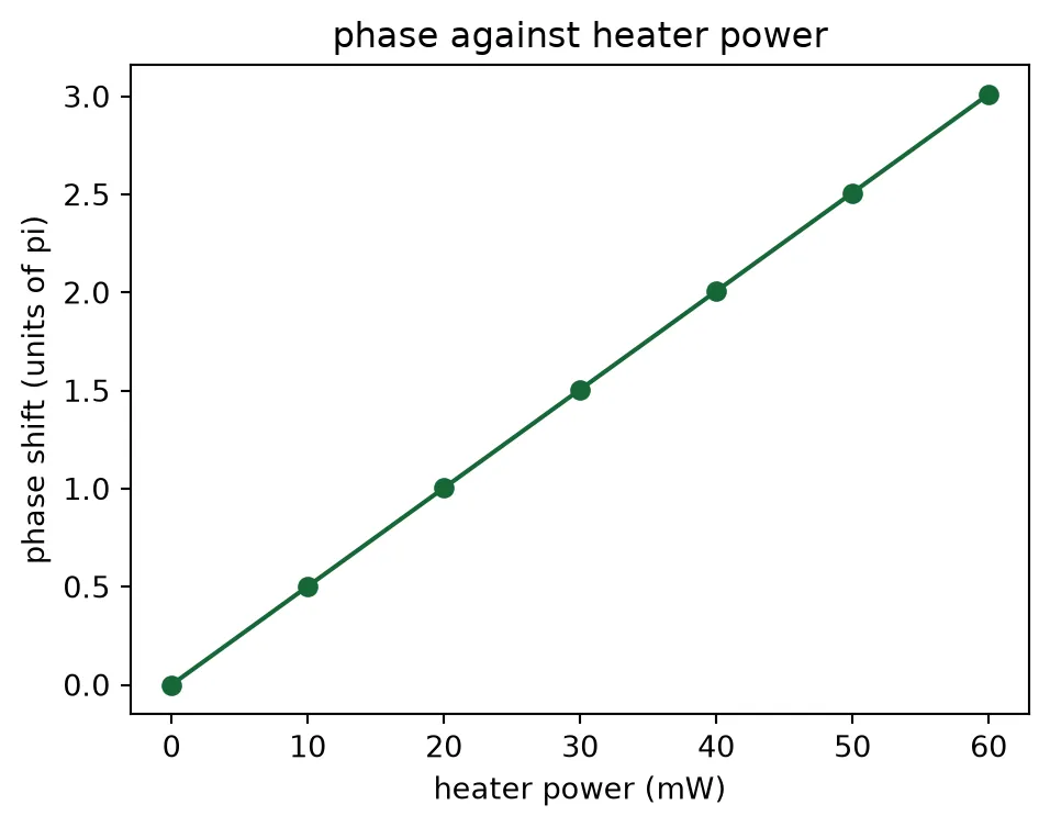

The detector, the edge coupler and the bond pad

The remaining cells are drawn here but not simulated, because their behaviour in the link is captured by a compact model and the physics behind each already has a worked example.

The germanium photodiode is a waveguide-coupled diode: light runs under a germanium block grown on the silicon and is absorbed over a few tens of microns. The receiver needs two of them, and what it needs from each is a responsivity, a bandwidth and a noise level, which is what the abstract photodiode block carries. The beat frequencies of this LiDAR are tens of megahertz, so the detector bandwidth is set to 1 GHz rather than the tens of gigahertz a data receiver needs, and the lower bandwidth buys a larger transimpedance gain.

The edge coupler is an inverse taper narrowing to a tip at the chip facet, and the Edge Coupler example works through simulating one. Here the geometry is kept and the facet enters the budget as the fixed 1.5 dB the system budget assumed.

The bond pad is where every heater net ends. A terminal alone defines a connection point without a shape; add_structure=True also draws the metal.

# 0.9 A/W is the responsivity the budget page derives its quantum efficiency from
@pf.parametric_component(name_prefix="PD")
def germanium_photodiode(
    *,
    length=25.0,
    ge_width=2.0,
    taper_length=10.0,
    responsivity=0.9,
    bandwidth=1e9,
    dark_current=10e-9,
    gain=1e4
):
    c = pf.Component()
    port_spec = pf.config.default_technology.ports["TE_1550_500"]

    # Silicon widens under the germanium so the mode transfers gradually, and reaches
    # out to one side to carry the anode plug
    c.add(
        "Si",
        pf.Path((-taper_length, 0), w_core)
        .segment((0, 0), width=ge_width)
        .segment((length, 0)),
        pf.Rectangle((0, -3.0), (length, 0)),
        # Germanium absorbs the light and generates the photocurrent
        "Ge",
        pf.Rectangle((0, -ge_width / 2), (length - 2, ge_width / 2)),
        # Anode plug on the silicon beside the germanium, cathode plug on top of it
        "Contact",
        pf.Rectangle((1, -2.8), (length - 1, -1.5)),
        "Ge Contact",
        pf.Rectangle((2, -0.5), (length - 4, 0.5)),
    )

    # The only strip facet is the narrow end of the taper, so detection finds the optical input
    c.add_port(c.detect_ports([port_spec]))
    # The photocurrent leaves on an electrical port, which a time stepper can read. No port
    # specification describes it, so it is placed by hand; the terminals below are for routing
    c.add_port(
        pf.Port((length, 0), 0, virtual_port_spec(classification="electrical")), "E0"
    )
    for name, y, sign in (("ANODE", -2.15, -1.0), ("CATHODE", 0.0, 1.0)):
        c.add_terminal(
            pf.Terminal(
                "M1",
                pf.Rectangle(
                    center=(length / 2 + sign * metal_width, y), size=(metal_width, 1.0)
                ),
            ),
            name,
            add_structure=True,
        )

    # The abstract photodiode carries responsivity, bandwidth and noise in two
    # models, optical and electrical. Grafting them gives the drawn cell physics.
    abstract_pd = pfa.photodiode(
        responsivity=responsivity,
        gain=gain,
        dark_current=dark_current,
        filter_frequency=bandwidth,
    )
    c.add_model(abstract_pd.models["Termination"], "pd", "optical")
    c.add_model(
        abstract_pd.models["Termination (electrical)"], "pd_electrical", "electrical"
    )
    return c

@pf.parametric_component(name_prefix="EC")
def edge_coupler(*, length=150.0, tip_width=0.18, insertion_loss=1.5):
    c = pf.Component()
    port_spec = pf.config.default_technology.ports["TE_1550_500"]
    # An inverse taper: the silicon narrows until the mode expands into the oxide
    c.add("Si", pf.Path((0, 0), tip_width).segment((length, 0), width=w_core))
    # The tip is not a strip, so detection would miss it; both ports are placed by hand
    # to keep the facet as P0
    c.add_port(pf.Port((0, 0), 0, port_spec), "P0")
    c.add_port(pf.Port((length, 0), 180, port_spec), "P1")
    c.add_model(pfa.edge_coupler(insertion_loss=insertion_loss).active_model, "facet")
    return c

# 50 um of metal, which is what a probe tip or a wire bond needs to land on
bond_pad = pf.Component("BondPad")
bond_pad.add_terminal(
    pf.Terminal("M1", pf.Rectangle(size=(50, 50))), add_structure=True
)
# The passivation opens 45 um across, leaving a 2.5 um rim of covered metal
bond_pad.add("Pad Open", pf.Rectangle(size=(45, 45)))

pd = germanium_photodiode()
ec = edge_coupler()
print("photodiode ports:", list(pd.ports), "terminals:", list(pd.terminals))
print("edge coupler ports:", list(ec.ports))
viewer(pd)

photodiode ports: ['E0', 'P0'] terminals: ['ANODE', 'CATHODE']
edge coupler ports: ['P0', 'P1']

The library

Nine cells, each with its own model. The chip pages place them and ask the assembly for an S matrix or drive it in time without knowing how any cell was characterized. The two antenna cells are the 20-period test sections of the antenna page; the chip layout page builds the full-length antennas from their measured periods and duty cycles.

library = {
    "antenna 500 nm": antenna_cell,
    "antenna 450 nm": second_cell,
    "1x2 splitter": splitter,
    "2x2 coupler": mixer,
    "LO tap": tap,
    "phase shifter": ps,
    "photodiode": pd,
    "edge coupler": ec,
    "bond pad": bond_pad,
}
print(f"{'cell':16s} {'ports':28s} {'terminals':22s} model")
for name, cell in library.items():
    print(
        f"{name:16s} {', '.join(cell.ports):28s} {', '.join(cell.terminals):22s} {cell.active_model_name}"
    )

cell             ports                        terminals              model
antenna 500 nm   P0, P1                                              FDTD
antenna 450 nm   P0, P1                                              FDTD
1x2 splitter     P0, P1, P2                                          EME
2x2 coupler      P0, P1, P2, P3                                      EME
LO tap           P0, P1, P2, P3                                      compact
phase shifter    P0, P1                       H0, H1                 thermal
photodiode       E0, P0                       ANODE, CATHODE         {'optical': 'pd', 'electrical': 'pd_electrical'}
edge coupler     P0, P1                                              facet
bond pad                                      T0                     None