

Paths, Routes, and Transitions
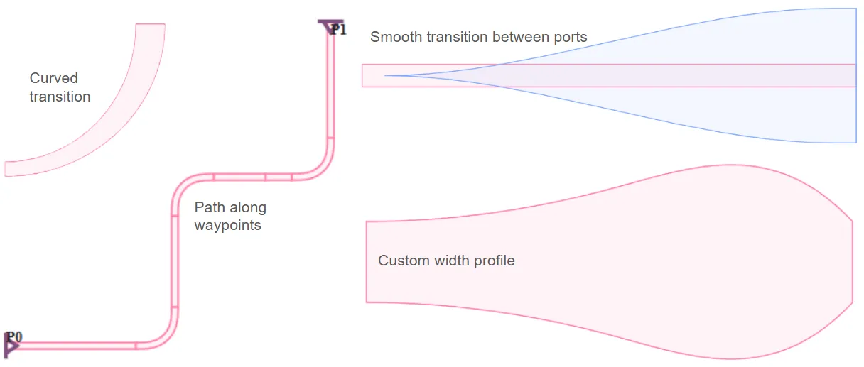
This notebook showcases the layout capabilities of PhotonForge for designing and manipulating photonic structures using paths. We cover how to define paths with varying widths and offsets, route between ports with or without waypoints, apply smooth transitions between different waveguide types, and generate envelopes and offset layers for fabrication. These tools provide a versatile foundation for creating complex photonic layouts with clarity and control.
import matplotlib.pyplot as pltimport numpy as npimport photonforge as pffrom photonforge.live_viewer import LiveViewer
viewer = LiveViewer()pf.config.default_technology = pf.basic_technology()
LiveViewer started at http://127.0.0.1:43091. Call its 'stop()' method to free the port.Creating a Path
Section titled “Creating a Path”We begin by creating a Path object. This structure allows us to define photonic waveguides, routes and even more complex structures. First, we add a straight segment, followed by an arc using the euler_fraction parameter to create a smooth curvature. Note that the arc angle is defined with respect to the y-axis in the clockwise direction.
# Create a new Path object starting at origin (0, 0) with initial width 0.5p = pf.Path(origin=(0, 0), width=0.5)
# Add a straight segment ending at (0, 5) with constant width 0.5p.segment(endpoint=(0, 5), width=0.5)
# Add a 45-degree arc (clockwise from y-axis), using Euler curvature smoothingp.arc(initial_angle=0, final_angle=45, radius=5, euler_fraction=0.5, width=0.5)
# Display the pathp
Let’s create a more advanced Path by chaining multiple segments and arcs. Note the following behaviors:
- If
widthis not specified insegmentorarc, the initial path width is used. - Setting
relative=Truemakes the endpoint relative to the current path position. - Angles in
arcare defined counter-clockwise from the x-axis, following the standard polar coordinate convention. However, the angles you specify inarc(initial_angle, final_angle)are interpreted with respect to the center of the arc. To produce a counter-clockwise turn, the final angle must be larger than the initial one. For example,arc(90, 180)creates a counter-clockwise bend.
# Create a complex Path by chaining arcs and segments
p = (    pf.Path((0, 0), width=0.5)  # Start at origin with width 0.5    .arc(-90, 0, radius=5)  # Clockwise arc from -90° to 0° with radius 5    .segment((0, 5), relative=True)  # Move up 5 units from the current position    .arc(180, 45, radius=3)  # Clockwise arc from 180° to 45° with radius 3    .segment((3, -3), relative=True)  # Move diagonally (relative to current position)    .arc(180 + 45, 180 + 90, radius=3)  # Counter-clockwise arc from 225° to 270°)
# Display the complex pathp
Using turn for Simpler Arc Definitions
Section titled “Using turn for Simpler Arc Definitions”We can simplify arc creation using the turn method, which only requires the turn angle and direction. Positive (negative) values make a counter-clockwise (clockwise) turn. This approach makes the code more readable and concise when building complex path geometries.
# Create a complex Path using turns and segments
p = (    pf.Path((0, 0), width=0.5)  # Start at origin with width 0.5    .turn(90, radius=5)  # Turn 90° clockwise with radius 5    .segment((0, 5), relative=True)  # Move up 5 units from the current position    .turn(-135, radius=3)  # Turn 135° counter-clockwise with radius 3    .segment((3, -3), relative=True)  # Move diagonally (relative to current position)    .turn(45, radius=3)  # Turn 45° clockwise with radius 3)
# Display the pathp
You can transform a path using chained methods:
copy()creates a duplicate of the original path.mirror()reflects the path across the x-axis.rotate(θ)rotates the path by θ degrees around the origin.translate((x, y))shifts the path by the specified vector.
or simply using transform() method (translate(rotate(mirror(scale(self))))).
# Equivalent to p2 = p.copy().transform(translation=(2, 0), rotation=45, scaling=1, x_reflection=True)p2 = p.copy().mirror().rotate(45).translate((2, 0))p2
You can also create an updated copy:
# Updated copy with new widthp3 = p.updated_copy(width=1)p3
To retrieve the central coordinates along a path, we can use the center() method. This returns an array of the centerline points, useful for analysis or plotting.
# Get the centerline coordinatescenter = p.center()x, y = zip(*center)  # Unpack into x and y lists
# Plot the centerlineplt.plot(x, y, marker=".")  # Plot points with markersplt.axis("equal")  # Equal aspect ratio for x and yplt.title("Path Centerline")plt.xlabel("x (µm)")plt.ylabel("y (µm)")plt.grid()plt.show()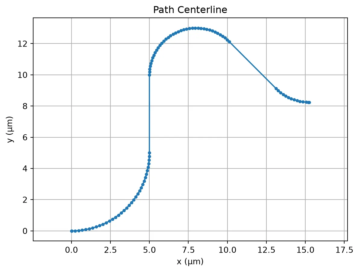
Accessing and Modifying Path Properties
Section titled “Accessing and Modifying Path Properties”Paths expose several geometric properties such as x_min, x_mid, x_max, y_min, y_mid, y_max, size, area, origin, and bounds(). These can be useful for alignment, placement, and inspection. Some of these properties are also settable; for example, we can shift the entire path vertically by updating y_min. The path length is another important property which can be calculated using length() method.
# Shift the path verticallyp.y_min += 2
# Get the centerline coordinatescenter = p.center()x, y = zip(*center)  # Unpack into x and y lists
# Plot the centerlineplt.plot(x, y, marker=".")  # Plot points with markersplt.axis("equal")  # Equal aspect ratio for x and yplt.title("Path Centerline")plt.xlabel("x (µm)")plt.ylabel("y (µm)")plt.grid()plt.show()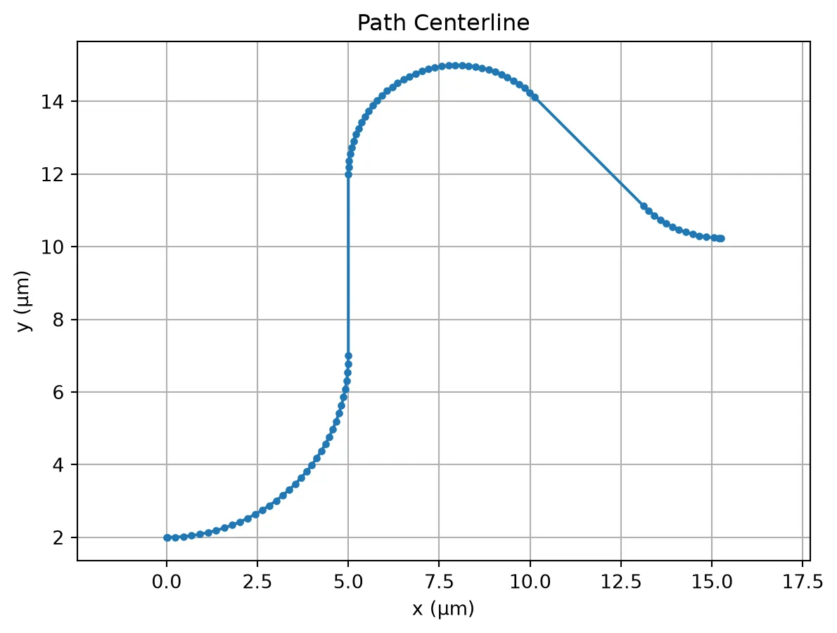
You can also check the length of the curve with the length() method:
# Print length of the pathprint(p.length())26.51931330563207Component Creation
Section titled “Component Creation”Now that you’ve got your path defined, the next step is to generate a Component. Then you can create 3D structures based on the extrusion specs of the default technology.
Option 1: Single layer and width cross section
Section titled “Option 1: Single layer and width cross section”The simplest option is to define a constant-width cross section and add it to a layer (e.g. the 220 nm “WG_CORE” layer) using the add method.
# Create a new Componentc = pf.Component()
# Add the path to the "WG_CORE" layer with default extrusion specsc.add("WG_CORE", p)
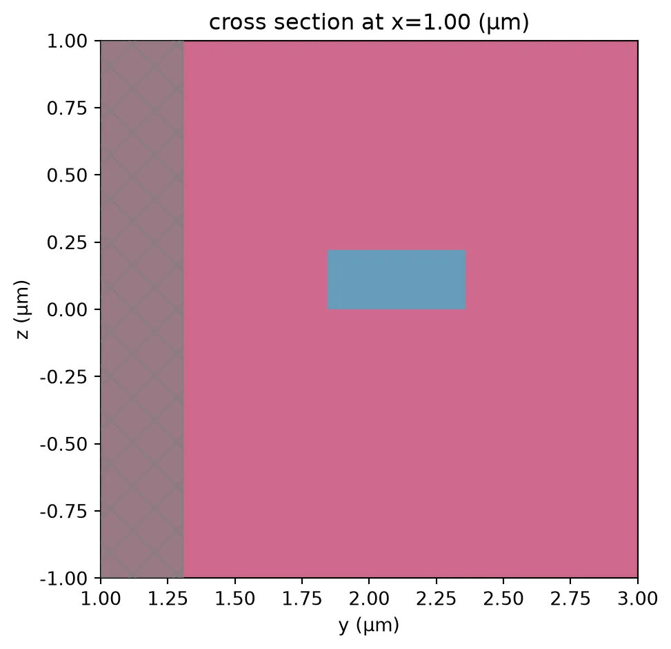
# Visualize the cross section of the 3D structure using the default Tidy3D plot settingspf.tidy3d_plot(c, x=1, vlim=(-1, 1), hlim=(1, 3))
# Display the component layoutc
Option 2: Multi-Layer Custom Cross Section
Section titled “Option 2: Multi-Layer Custom Cross Section”You can also define an arbitrary cross section by stacking multiple paths on different layers. This allows you to model structures like a “Rib” waveguide. In this example, we create a narrow core on the “WG_CORE” layer and a wider slab on the “SLAB” layer.
# Create the core waveguide pathp1 = pf.Path((0, 0), width=0.5).segment((5, 0))
# Create the slab pathp2 = pf.Path((0, 0), width=5).segment((5, 0))
# Create a new Componentc = pf.Component()
# Add the paths to different layers: core on "WG_CORE", slab on "SLAB"c.add("WG_CORE", p1, "SLAB", p2)
# Visualize the cross section of the resulting 3D structurepf.tidy3d_plot(c, x=1, vlim=(-1, 1), hlim=(-3, 3))
# Display the component layoutc
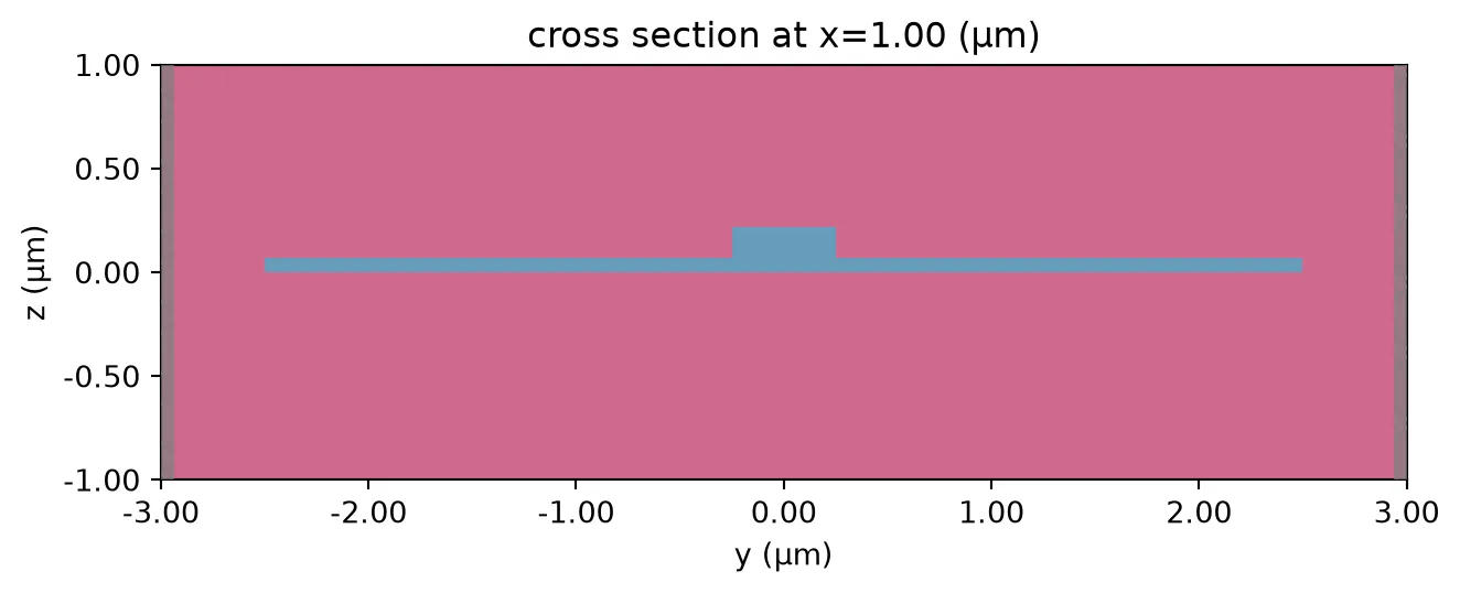
You can also assign an offset to the path. Let’s apply an offset to the slab path in the previous example.
# Create the waveguide path with offsetp1 = pf.Path((0, 0), width=0.5, offset=3).segment((5, 0))
# Create a new Componentc = pf.Component()
# Add the paths to different layers: core on "WG_CORE", slab on "SLAB"c.add("WG_CORE", p1, "SLAB", p2)
The offset of a path can vary along its length. You can define the offset change using a constant value, a smooth transition, or a custom expression. In this example, the offset varies linearly from 3 to 4 along the segment.
# Create a path with width 0.5 and varying offsetp1 = pf.Path((0, 0), width=0.5).segment((5, 0), offset=(3, 4, "linear"))
# Create a new Componentc = pf.Component()
# Add the paths to different layers: core on "WG_CORE", slab on "SLAB"c.add("WG_CORE", p1, "SLAB", p2)
Option 3: Tapered Cross Section
Section titled “Option 3: Tapered Cross Section”You can create tapered waveguides by specifying a varying width along the segment. By default, the interpolation is linear, but you can also choose "smooth" for a gradual transition using a third-degree polynomial with zero derivatives at both ends. Additionally, you can modify the starting width if needed.
# Create a tapered path from width 0.5 to 1 using smooth interpolationp = pf.Path((0, 0), width=0.5).segment((3, 0), width=(1, "smooth"))
# Create a new Componentc = pf.Component()
# Add the tapered path to the "WG_CORE" layerc.add("WG_CORE", p)
Tapering Along a Curved Path
Tapering is not limited to straight segments—it can also be applied along curves. In this example, we create a 90° turn and taper the width smoothly from 0.5 to 1 along the arc.
p = pf.Path((0, 0), width=0.5).turn(90, radius=5, width=(1, "smooth"))
# Create a new Componentc = pf.Component()
# Add the tapered path to the "WG_CORE" layerc.add("WG_CORE", p)
For full control over the taper profile, you can define a custom width using an expression pair: (value_expression, derivative_expression). These are evaluated along the segment using the variable u, which ranges from 0 to 1 along the path. This allows for arbitrary taper shapes and smoothness. Refer to the documentation on Expression for supported syntax and operators.
# Create a path with width defined by a custom expressionp = pf.Path((0, 0), width=0.5).segment((3, 0), ("0.5 + 0.5 * u^2", "u"))
# Create a new Componentc = pf.Component()
# Add the custom-tapered path to the "WG_CORE" layerc.add("WG_CORE", p)
Option 4: Cross Section with Custom Width Profile
Section titled “Option 4: Cross Section with Custom Width Profile”This approach is useful in many photonic devices for designing adiabatic tapers. Here, we define a width profile using cubic spline interpolation and apply it segment-by-segment along the path. This allows for a smooth and highly customized transition of waveguide width.
from scipy.interpolate import make_interp_spline
# Define control widths and total taper lengthwidth_ctrl = [0.5, 0.6, 0.9, 1.2, 0.5]length = 3
# Create a smooth spline curve from the control pointsx_ctrl = np.linspace(0, length, len(width_ctrl))spline = make_interp_spline(x_ctrl, width_ctrl, k=3)
# Generate high-resolution points along the splinex_dense = np.linspace(0, length, 100)widths = spline(x_dense)
# Construct the path using the interpolated width profilep = pf.Path((0, 0), width=widths[0])for x, w in zip(x_dense[1:], widths[1:]):    p.segment((x, 0), w)
# Create a component and add the pathc = pf.Component()c.add("WG_CORE", p)
# Display the resultc
Option 5: Putting Components Along the Path
Section titled “Option 5: Putting Components Along the Path”In some applications, we may want to place a repeated structure—like electrodes or teeth—along a transmission line or waveguide path. Here we demonstrate how to define such a pattern using a zero-width path and a custom parametric section. We then design a simple “tooth” component and use the interpolate method to place copies of it periodically along the path, while aligning them with the local tangent direction. This is especially useful for building segmented coplanar waveguides (CPW), grating waveguides, or periodic electrodes/vias.
# Create a path with zero width, composed of segments and parametric curvesp = ( pf.Path((0, 0), 0) # Start with zero width .segment((50, 0)) # Straight segment to the right .s_bend((180, 20), euler_fraction=0.5) # Smooth 180° turn .parametric( # Add a parametric curve section ("80 * u", "-40 * u^2"), # Parametric x(u), y(u) ("80", "-80 * u"), # Derivative dx/du, dy/du ))# Create a basic "tooth" structure using rectangles on the METAL layertooth = pf.Component("Tooth")
tooth.add( "METAL", pf.Rectangle((-0.5, -1.3), (0.5, -0.5)), # Narrow vertical finger (bottom) pf.Rectangle((-3, -0.5), (3, -0.2)), # Horizontal plate (bottom) pf.Rectangle((-0.5, 1.3), (0.5, 0.5)), # Narrow vertical finger (top) pf.Rectangle((-3, 0.5), (3, 0.2)), # Horizontal plate (top))
# Create a CPW tooth component by duplicating the base tooth above and below the CPW centercpw_tooth = pf.Component("Cpw Tooth")cpw_tooth.add_reference(tooth).translate((0, 3.05)) # Top electrodecpw_tooth.add_reference(tooth).translate((0, -3.05)) # Bottom electrode
# Display the CPW tooth componentcpw_tooth;fill:%23221f20;font-weight:bold;font-size:0.382800px;}.terminal{fill:none;stroke:%23805080;stroke-width:0.047850;}.dashed{stroke-dasharray:0.239250,0.143550;}.port{fill:none;stroke:%23805080;stroke-width:0.095700;}.virtual-connection{fill:none;stroke:%23907090;stroke-width:0.071775;}.layer_5_0{stroke:%23998573;fill:url(%23pat-layer_5_0);fill-opacity:0.492;}.label_5_0{fill:%23998573;}.layer_3_0{stroke:%238851ad;fill:url(%23pat-layer_3_0);fill-opacity:0.492;}.label_3_0{fill:%238851ad;}.layer_4_0{stroke:%23535e59;fill:url(%23pat-layer_4_0);fill-opacity:0.492;}.label_4_0{fill:%23535e59;}.layer_1_0{stroke:%23858d89;fill:url(%23pat-layer_1_0);fill-opacity:0.492;}.label_1_0{fill:%23858d89;}.layer_2_0{stroke:%235b98b9;fill:url(%23pat-layer_2_0);fill-opacity:0.492;}.label_2_0{fill:%235b98b9;}</style><defs><path id=%22port-symbol%22 class=%22port%22 d=%22M 0,-0.191400 L 0.287100,0 0,0.191400%22 /><path id=%22ref-port-symbol%22 class=%22port%22 style=%22stroke-opacity:0.33;%22 d=%22M 0,-0.143550 C 0.191400,-0.143550 0.191400,0.143550 0,0.143550%22 /><circle id=%22port-bend-symbol%22 style=%22stroke-width:0;stroke:none;fill:%23805080;fill-opacity:1;%22 cx=%220%22 cy=%220%22 r=%220.086130%22 /><circle id=%22connection-symbol%22 style=%22stroke-width:0;stroke:none;fill:%23907090;fill-opacity:1;%22 cx=%220%22 cy=%220%22 r=%220.100485%22 /><pattern id=%22pat-layer_5_0%22 patternUnits=%22userSpaceOnUse%22 width=%220.239250%22 height=%220.239250%22 patternTransform=%22translate(0.014074,0.214066)%22><line x1=%220.239250%22 y1=%220%22 x2=%220%22 y2=%220.239250%22 style=%22stroke:%23998573;stroke-width:0.023925%22 /><line x1=%220.358875%22 y1=%220.119625%22 x2=%220.119625%22 y2=%220.358875%22 style=%22stroke:%23998573;stroke-width:0.023925%22 /><line x1=%220.119625%22 y1=%22-0.119625%22 x2=%22-0.119625%22 y2=%220.119625%22 style=%22stroke:%23998573;stroke-width:0.023925%22 /></pattern><pattern id=%22pat-layer_3_0%22 patternUnits=%22userSpaceOnUse%22 width=%220.143550%22 height=%220.143550%22 patternTransform=%22translate(0.033776,0.105774)%22><circle cx=%220.071775%22 cy=%220.071775%22 r=%220.023925%22 style=%22stroke:none;fill:%238851ad;fill-opacity:1.0%22 /></pattern><pattern id=%22pat-layer_4_0%22 patternUnits=%22userSpaceOnUse%22 width=%220.239250%22 height=%220.239250%22 patternTransform=%22translate(0.154809,0.075553)%22><line x1=%220.119625%22 y1=%220%22 x2=%220.119625%22 y2=%220.239250%22 style=%22stroke:%23535e59;stroke-width:0.023925%22 /><line x1=%220%22 y1=%220.119625%22 x2=%220.239250%22 y2=%220.119625%22 style=%22stroke:%23535e59;stroke-width:0.023925%22 /></pattern><pattern id=%22pat-layer_1_0%22 patternUnits=%22userSpaceOnUse%22 width=%220.239250%22 height=%220.239250%22 patternTransform=%22translate(0.098515,0.138513)%22><circle cx=%220.119625%22 cy=%220.119625%22 r=%220.023925%22 style=%22stroke:none;fill:%23858d89;fill-opacity:1.0%22 /></pattern><pattern id=%22pat-layer_2_0%22 patternUnits=%22userSpaceOnUse%22 width=%220.239250%22 height=%220.239250%22 patternTransform=%22translate(0.197029,0.037776)%22><line x1=%220%22 y1=%220%22 x2=%220.239250%22 y2=%220.239250%22 style=%22stroke:%235b98b9;stroke-width:0.023925%22 /><line x1=%22-0.119625%22 y1=%220.119625%22 x2=%220.119625%22 y2=%220.358875%22 style=%22stroke:%235b98b9;stroke-width:0.023925%22 /><line x1=%220.119625%22 y1=%22-0.119625%22 x2=%220.358875%22 y2=%220.119625%22 style=%22stroke:%235b98b9;stroke-width:0.023925%22 /></pattern><g id=%22C1%22 data-name=%22Tooth%22><rect class=%22layer_5_0%22 x=%22-0.500000%22 y=%22-1.300000%22 width=%221.000000%22 height=%220.800000%22 /><rect class=%22layer_5_0%22 x=%22-3.000000%22 y=%22-0.500000%22 width=%226.000000%22 height=%220.300000%22 /><rect class=%22layer_5_0%22 x=%22-0.500000%22 y=%220.500000%22 width=%221.000000%22 height=%220.800000%22 /><rect class=%22layer_5_0%22 x=%22-3.000000%22 y=%220.200000%22 width=%226.000000%22 height=%220.300000%22 /></g></defs><g transform=%22scale(1 -1)%22><g id=%22C0%22 data-name=%22Cpw Tooth%22><use transform=%22translate(0.000000 3.050000)%22 href=%22%23C1%22 /><use transform=%22translate(0.000000 -3.050000)%22 href=%22%23C1%22 /></g></g></svg>)
%22><rect x=%22-30.00%22 y=%22-30.00%22 width=%2260.00%22 height=%2260.00%22 fill=%22%23f4f5f7%22 stroke=%22%23232530%22 stroke-width=%221%22/></g><text x=%2240.00%22 y=%2240.00%22 font-size=%226.5%22 fill=%22%23232530%22 font-weight=%22400%22 text-anchor=%22middle%22 dominant-baseline=%22middle%22 stroke=%22%23ffffff%22 stroke-width=%222.27%22 stroke-linejoin=%22round%22 paint-order=%22stroke%22>Tooth</text><text x=%2240.00%22 y=%2271.80%22 font-size=%229%22 fill=%22%23232530%22 font-weight=%22400%22 text-anchor=%22middle%22 dominant-baseline=%22hanging%22 stroke=%22%23ffffff%22 stroke-width=%223.15%22 stroke-linejoin=%22round%22 paint-order=%22stroke%22>Tooth_1</text><g transform=%22matrix(1 -0 0 1 40.000 200.000)%22><rect x=%22-30.00%22 y=%22-30.00%22 width=%2260.00%22 height=%2260.00%22 fill=%22%23f4f5f7%22 stroke=%22%23232530%22 stroke-width=%221%22/></g><text x=%2240.00%22 y=%22200.00%22 font-size=%226.5%22 fill=%22%23232530%22 font-weight=%22400%22 text-anchor=%22middle%22 dominant-baseline=%22middle%22 stroke=%22%23ffffff%22 stroke-width=%222.27%22 stroke-linejoin=%22round%22 paint-order=%22stroke%22>Tooth</text><text x=%2240.00%22 y=%22231.80%22 font-size=%229%22 fill=%22%23232530%22 font-weight=%22400%22 text-anchor=%22middle%22 dominant-baseline=%22hanging%22 stroke=%22%23ffffff%22 stroke-width=%223.15%22 stroke-linejoin=%22round%22 paint-order=%22stroke%22>Tooth_2</text><g fill=%22none%22 stroke-width=%222%22></g></svg>)
# Function to extrude a port profile along a path and place periodic componentsdef extrude(    path: pf.Path, port_spec: pf.PortSpec, period: float = 0, reference=None) -> pf.Component:    c = pf.Component()  # Create a new component to hold the result
    # Add base paths to the appropriate layers    for width, offset, layer in port_spec.path_profiles_list():        c.add(layer, path.updated_copy(width, offset))
    # If a periodic component reference is provided, place it along the path    if period > 0 and reference is not None:        if isinstance(reference, pf.Component):            reference = pf.Reference(reference)
        # Determine positions along the path and place aligned copies        s = np.arange(period / 2, path.length(), period)        for position, _, _, grad in zip(*path.interpolate(s)):            rotation = np.arctan2(grad[1], grad[0]) * 180.0 / np.pi            c.add(reference.copy().transform(position, rotation))
    return c
# Extrude the CPW line and place teeth periodically along the pathcpw = pf.cpw_spec("METAL", 3.6, 2.6)c = extrude( path=p, # Path to follow port_spec=cpw, # CPW port spec period=10, # Periodic placement every 10 µm reference=cpw_tooth, # Component to place along path)
# Display the final component with path and teethviewer(c);fill:%23221f20;font-weight:bold;font-size:4.995696px;}.terminal{fill:none;stroke:%23805080;stroke-width:0.624462;}.dashed{stroke-dasharray:3.122310,1.873386;}.port{fill:none;stroke:%23805080;stroke-width:1.248924;}.virtual-connection{fill:none;stroke:%23907090;stroke-width:0.936693;}.layer_5_0{stroke:%23998573;fill:url(%23pat-layer_5_0);fill-opacity:0.492;}.label_5_0{fill:%23998573;}.layer_3_0{stroke:%238851ad;fill:url(%23pat-layer_3_0);fill-opacity:0.492;}.label_3_0{fill:%238851ad;}.layer_4_0{stroke:%23535e59;fill:url(%23pat-layer_4_0);fill-opacity:0.492;}.label_4_0{fill:%23535e59;}.layer_1_0{stroke:%23858d89;fill:url(%23pat-layer_1_0);fill-opacity:0.492;}.label_1_0{fill:%23858d89;}.layer_2_0{stroke:%235b98b9;fill:url(%23pat-layer_2_0);fill-opacity:0.492;}.label_2_0{fill:%235b98b9;}</style><defs><path id=%22port-symbol%22 class=%22port%22 d=%22M 0,-2.497848 L 3.746772,0 0,2.497848%22 /><path id=%22ref-port-symbol%22 class=%22port%22 style=%22stroke-opacity:0.33;%22 d=%22M 0,-1.873386 C 2.497848,-1.873386 2.497848,1.873386 0,1.873386%22 /><circle id=%22port-bend-symbol%22 style=%22stroke-width:0;stroke:none;fill:%23805080;fill-opacity:1;%22 cx=%220%22 cy=%220%22 r=%221.124032%22 /><circle id=%22connection-symbol%22 style=%22stroke-width:0;stroke:none;fill:%23907090;fill-opacity:1;%22 cx=%220%22 cy=%220%22 r=%221.311370%22 /><pattern id=%22pat-layer_5_0%22 patternUnits=%22userSpaceOnUse%22 width=%223.122310%22 height=%223.122310%22 patternTransform=%22translate(0.183665,2.793646)%22><line x1=%223.122310%22 y1=%220%22 x2=%220%22 y2=%223.122310%22 style=%22stroke:%23998573;stroke-width:0.312231%22 /><line x1=%224.683465%22 y1=%221.561155%22 x2=%221.561155%22 y2=%224.683465%22 style=%22stroke:%23998573;stroke-width:0.312231%22 /><line x1=%221.561155%22 y1=%22-1.561155%22 x2=%22-1.561155%22 y2=%221.561155%22 style=%22stroke:%23998573;stroke-width:0.312231%22 /></pattern><pattern id=%22pat-layer_3_0%22 patternUnits=%22userSpaceOnUse%22 width=%221.873386%22 height=%221.873386%22 patternTransform=%22translate(0.440797,1.380390)%22><circle cx=%220.936693%22 cy=%220.936693%22 r=%220.312231%22 style=%22stroke:none;fill:%238851ad;fill-opacity:1.0%22 /></pattern><pattern id=%22pat-layer_4_0%22 patternUnits=%22userSpaceOnUse%22 width=%223.122310%22 height=%223.122310%22 patternTransform=%22translate(2.020318,0.985993)%22><line x1=%221.561155%22 y1=%220%22 x2=%221.561155%22 y2=%223.122310%22 style=%22stroke:%23535e59;stroke-width:0.312231%22 /><line x1=%220%22 y1=%221.561155%22 x2=%223.122310%22 y2=%221.561155%22 style=%22stroke:%23535e59;stroke-width:0.312231%22 /></pattern><pattern id=%22pat-layer_1_0%22 patternUnits=%22userSpaceOnUse%22 width=%223.122310%22 height=%223.122310%22 patternTransform=%22translate(1.285657,1.807653)%22><circle cx=%221.561155%22 cy=%221.561155%22 r=%220.312231%22 style=%22stroke:none;fill:%23858d89;fill-opacity:1.0%22 /></pattern><pattern id=%22pat-layer_2_0%22 patternUnits=%22userSpaceOnUse%22 width=%223.122310%22 height=%223.122310%22 patternTransform=%22translate(2.571314,0.492996)%22><line x1=%220%22 y1=%220%22 x2=%223.122310%22 y2=%223.122310%22 style=%22stroke:%235b98b9;stroke-width:0.312231%22 /><line x1=%22-1.561155%22 y1=%221.561155%22 x2=%221.561155%22 y2=%224.683465%22 style=%22stroke:%235b98b9;stroke-width:0.312231%22 /><line x1=%221.561155%22 y1=%22-1.561155%22 x2=%224.683465%22 y2=%221.561155%22 style=%22stroke:%235b98b9;stroke-width:0.312231%22 /></pattern><g id=%22C1%22 data-name=%22Cpw Tooth%22><use transform=%22translate(0.000000 3.050000)%22 href=%22%23C2%22 /><use transform=%22translate(0.000000 -3.050000)%22 href=%22%23C2%22 /></g><g id=%22C2%22 data-name=%22Tooth%22><rect class=%22layer_5_0%22 x=%22-0.500000%22 y=%22-1.300000%22 width=%221.000000%22 height=%220.800000%22 /><rect class=%22layer_5_0%22 x=%22-3.000000%22 y=%22-0.500000%22 width=%226.000000%22 height=%220.300000%22 /><rect class=%22layer_5_0%22 x=%22-0.500000%22 y=%220.500000%22 width=%221.000000%22 height=%220.800000%22 /><rect class=%22layer_5_0%22 x=%22-3.000000%22 y=%220.200000%22 width=%226.000000%22 height=%220.300000%22 /></g></defs><g transform=%22scale(1 -1)%22><g id=%22C0%22><use transform=%22translate(5.000000 0.000000)%22 href=%22%23C1%22 /><use transform=%22translate(15.000000 0.000000)%22 href=%22%23C1%22 /><use transform=%22translate(25.000000 0.000000)%22 href=%22%23C1%22 /><use transform=%22translate(35.000000 0.000000)%22 href=%22%23C1%22 /><use transform=%22translate(45.000000 0.000000)%22 href=%22%23C1%22 /><use transform=%22translate(55.000000 0.006500) rotate(0.224844)%22 href=%22%23C1%22 /><use transform=%22translate(64.998000 0.176500) rotate(2.023517)%22 href=%22%23C1%22 /><use transform=%22translate(74.976500 0.815500) rotate(5.542726)%22 href=%22%23C1%22 /><use transform=%22translate(84.888500 2.125000) rotate(9.509058)%22 href=%22%23C1%22 /><use transform=%22translate(94.686000 4.117000) rotate(13.468046)%22 href=%22%23C1%22 /><use transform=%22translate(104.340500 6.717000) rotate(16.373523)%22 href=%22%23C1%22 /><use transform=%22translate(113.900000 9.653500) rotate(17.480358)%22 href=%22%23C1%22 /><use transform=%22translate(123.448500 12.624500) rotate(16.788480)%22 href=%22%23C1%22 /><use transform=%22translate(133.074500 15.329000) rotate(14.297982)%22 href=%22%23C1%22 /><use transform=%22translate(142.839500 17.475500) rotate(10.424087)%22 href=%22%23C1%22 /><use transform=%22translate(152.729500 18.943000) rotate(6.457719)%22 href=%22%23C1%22 /><use transform=%22translate(162.697000 19.729000) rotate(2.693747)%22 href=%22%23C1%22 /><use transform=%22translate(172.693000 19.979500) rotate(0.480187)%22 href=%22%23C1%22 /><use transform=%22translate(182.692500 19.954500) rotate(-1.927642)%22 href=%22%23C1%22 /><use transform=%22translate(192.640500 19.001500) rotate(-8.978938)%22 href=%22%23C1%22 /><use transform=%22translate(202.403500 16.863000) rotate(-15.644635)%22 href=%22%23C1%22 /><use transform=%22translate(211.868500 13.652500) rotate(-21.720225)%22 href=%22%23C1%22 /><use transform=%22translate(220.966500 9.511000) rotate(-27.116224)%22 href=%22%23C1%22 /><use transform=%22translate(229.665000 4.583500) rotate(-31.832609)%22 href=%22%23C1%22 /><use transform=%22translate(237.960500 -0.996500) rotate(-35.923617)%22 href=%22%23C1%22 /><use transform=%22translate(245.868000 -7.116000) rotate(-39.466234)%22 href=%22%23C1%22 /><use transform=%22translate(253.409500 -13.681000) rotate(-42.540074)%22 href=%22%23C1%22 /><path class=%22layer_5_0%22 d=%22M 0.000000,-33.126000 50.000000,-33.126000 54.224000,-33.122000 58.625000,-33.094000 60.892000,-33.063000 63.203000,-33.016000 65.558000,-32.949000 67.957000,-32.859000 70.399000,-32.740000 72.884000,-32.589000 75.409000,-32.402000 76.675000,-32.295000 79.205000,-32.053000 81.731000,-31.774000 84.253000,-31.460000 86.770000,-31.109000 88.026000,-30.921000 90.535000,-30.516000 91.787000,-30.301000 94.287000,-29.842000 96.780000,-29.349000 99.266000,-28.819000 101.743000,-28.254000 104.184000,-27.662000 106.574000,-27.049000 108.914000,-26.421000 111.204000,-25.781000 113.447000,-25.134000 115.642000,-24.482000 117.790000,-23.831000 121.951000,-22.540000 124.957000,-21.594000 128.817000,-20.381000 132.513000,-19.242000 134.301000,-18.705000 136.051000,-18.192000 137.761000,-17.706000 139.434000,-17.248000 141.068000,-16.819000 142.664000,-16.420000 144.224000,-16.053000 145.780000,-15.709000 147.341000,-15.389000 148.906000,-15.090000 150.475000,-14.814000 152.048000,-14.561000 153.624000,-14.330000 155.204000,-14.121000 156.786000,-13.936000 158.371000,-13.772000 159.958000,-13.632000 161.557000,-13.514000 163.199000,-13.414000 164.886000,-13.332000 166.619000,-13.267000 168.397000,-13.216000 170.219000,-13.179000 173.998000,-13.138000 176.949000,-13.127000 180.000000,-13.126000 180.732000,-13.132000 181.465000,-13.149000 182.199000,-13.177000 183.670000,-13.269000 184.408000,-13.333000 185.148000,-13.408000 185.891000,-13.495000 186.637000,-13.594000 187.386000,-13.705000 188.139000,-13.829000 188.895000,-13.965000 189.656000,-14.113000 190.421000,-14.275000 191.191000,-14.449000 191.966000,-14.637000 192.746000,-14.838000 193.531000,-15.053000 194.322000,-15.281000 195.119000,-15.524000 195.922000,-15.781000 196.731000,-16.053000 197.547000,-16.340000 198.369000,-16.642000 199.197000,-16.959000 200.032000,-17.292000 200.874000,-17.640000 201.723000,-18.005000 202.578000,-18.386000 203.440000,-18.783000 204.309000,-19.197000 205.186000,-19.629000 206.069000,-20.077000 206.959000,-20.543000 207.856000,-21.027000 208.760000,-21.528000 209.670000,-22.047000 210.588000,-22.585000 211.512000,-23.141000 212.443000,-23.716000 213.381000,-24.309000 214.325000,-24.921000 215.276000,-25.553000 216.233000,-26.203000 217.197000,-26.873000 218.167000,-27.563000 219.142000,-28.272000 220.124000,-29.001000 221.112000,-29.749000 222.106000,-30.518000 223.106000,-31.307000 224.111000,-32.116000 225.122000,-32.945000 226.138000,-33.794000 227.160000,-34.664000 228.186000,-35.555000 229.218000,-36.466000 230.255000,-37.397000 231.297000,-38.350000 232.344000,-39.323000 233.395000,-40.317000 234.451000,-41.331000 235.512000,-42.367000 236.576000,-43.424000 256.889000,-23.111000 255.663000,-21.895000 254.439000,-20.699000 253.214000,-19.523000 251.991000,-18.366000 250.768000,-17.229000 249.545000,-16.112000 248.324000,-15.014000 247.103000,-13.936000 245.882000,-12.878000 244.663000,-11.839000 243.444000,-10.820000 242.225000,-9.821000 241.008000,-8.841000 239.791000,-7.881000 238.575000,-6.941000 237.360000,-6.020000 236.146000,-5.119000 234.932000,-4.237000 233.719000,-3.375000 232.507000,-2.532000 231.296000,-1.709000 230.086000,-0.905000 228.877000,-0.121000 227.668000,0.644000 226.460000,1.389000 225.254000,2.115000 224.048000,2.822000 222.843000,3.509000 221.639000,4.177000 220.436000,4.825000 219.234000,5.455000 218.032000,6.065000 216.832000,6.655000 215.632000,7.227000 214.434000,7.779000 213.236000,8.313000 212.040000,8.827000 210.844000,9.322000 209.649000,9.798000 208.455000,10.255000 207.262000,10.693000 206.070000,11.112000 204.878000,11.513000 203.688000,11.894000 202.498000,12.257000 201.309000,12.600000 200.120000,12.925000 198.933000,13.231000 197.746000,13.519000 196.560000,13.788000 195.374000,14.038000 194.189000,14.269000 193.005000,14.482000 191.821000,14.676000 190.637000,14.852000 189.454000,15.009000 188.272000,15.148000 187.089000,15.268000 185.907000,15.369000 184.726000,15.452000 183.544000,15.517000 182.363000,15.563000 181.181000,15.591000 180.000000,15.600000 175.877000,15.596000 171.778000,15.571000 169.738000,15.543000 167.703000,15.501000 165.675000,15.444000 163.653000,15.367000 161.639000,15.270000 159.631000,15.148000 157.631000,14.999000 155.635000,14.823000 153.641000,14.618000 151.650000,14.384000 149.663000,14.122000 147.680000,13.831000 145.701000,13.512000 143.727000,13.165000 141.758000,12.790000 139.795000,12.386000 137.838000,11.954000 135.885000,11.495000 133.934000,11.007000 131.983000,10.495000 130.032000,9.960000 128.080000,9.406000 126.128000,8.834000 124.173000,8.247000 120.256000,7.039000 116.323000,5.803000 112.367000,4.561000 108.382000,3.332000 106.376000,2.730000 104.361000,2.140000 102.336000,1.564000 100.299000,1.006000 98.251000,0.468000 96.191000,-0.046000 94.119000,-0.534000 92.039000,-0.993000 89.952000,-1.422000 87.859000,-1.821000 85.761000,-2.190000 83.658000,-2.529000 81.551000,-2.838000 79.439000,-3.116000 77.323000,-3.365000 75.204000,-3.583000 73.082000,-3.771000 70.959000,-3.928000 68.839000,-4.057000 66.724000,-4.159000 64.614000,-4.239000 62.509000,-4.299000 60.410000,-4.342000 58.316000,-4.370000 54.146000,-4.396000 50.000000,-4.400000 0.000000,-4.400000 z%22 /><path class=%22layer_5_0%22 d=%22M 0.000000,4.400000 50.000000,4.400000 54.123000,4.404000 58.222000,4.429000 60.262000,4.457000 62.297000,4.499000 64.325000,4.556000 66.347000,4.633000 68.361000,4.730000 70.369000,4.852000 72.369000,5.001000 74.365000,5.177000 76.359000,5.382000 78.350000,5.616000 80.337000,5.878000 82.320000,6.169000 84.299000,6.488000 86.273000,6.835000 88.242000,7.210000 90.205000,7.614000 92.162000,8.046000 94.115000,8.505000 96.066000,8.993000 98.017000,9.505000 99.968000,10.040000 101.920000,10.594000 103.872000,11.166000 105.827000,11.753000 109.744000,12.961000 113.677000,14.197000 117.633000,15.439000 121.618000,16.668000 123.624000,17.270000 125.639000,17.860000 127.664000,18.436000 129.701000,18.994000 131.749000,19.532000 133.809000,20.046000 135.881000,20.534000 137.961000,20.993000 140.048000,21.422000 142.141000,21.821000 144.239000,22.190000 146.342000,22.529000 148.449000,22.838000 150.561000,23.116000 152.677000,23.365000 154.796000,23.583000 156.918000,23.771000 159.041000,23.928000 161.161000,24.057000 163.276000,24.159000 165.386000,24.239000 167.491000,24.299000 169.590000,24.342000 171.684000,24.370000 175.854000,24.396000 180.000000,24.400000 181.319000,24.390000 182.637000,24.359000 183.956000,24.307000 185.274000,24.235000 186.593000,24.143000 187.911000,24.029000 189.228000,23.895000 190.546000,23.741000 191.863000,23.566000 193.179000,23.371000 194.495000,23.155000 195.811000,22.918000 197.126000,22.662000 198.440000,22.384000 199.754000,22.087000 201.067000,21.769000 202.380000,21.430000 203.691000,21.072000 205.002000,20.693000 206.312000,20.293000 207.622000,19.874000 208.930000,19.434000 210.238000,18.975000 211.545000,18.495000 212.851000,17.995000 214.156000,17.475000 215.460000,16.935000 216.764000,16.375000 218.066000,15.795000 219.368000,15.195000 220.668000,14.575000 221.968000,13.935000 223.266000,13.276000 224.564000,12.597000 225.861000,11.898000 227.157000,11.179000 228.452000,10.440000 229.746000,9.682000 231.040000,8.904000 232.332000,8.106000 233.623000,7.289000 234.914000,6.452000 236.204000,5.596000 237.493000,4.720000 238.781000,3.824000 240.068000,2.909000 241.354000,1.974000 242.640000,1.020000 243.925000,0.046000 245.209000,-0.947000 246.492000,-1.959000 247.775000,-2.991000 249.056000,-4.043000 250.337000,-5.114000 251.618000,-6.204000 252.897000,-7.314000 254.176000,-8.443000 255.455000,-9.591000 256.732000,-10.759000 258.009000,-11.946000 259.286000,-13.153000 260.562000,-14.379000 261.837000,-15.624000 263.111000,-16.889000 283.424000,3.424000 281.988000,4.847000 280.549000,6.253000 279.105000,7.641000 277.656000,9.010000 276.203000,10.361000 274.745000,11.694000 273.282000,13.009000 271.814000,14.305000 270.340000,15.582000 268.862000,16.841000 267.378000,18.082000 265.889000,19.303000 264.394000,20.506000 262.894000,21.690000 261.388000,22.855000 259.876000,24.001000 258.358000,25.127000 256.833000,26.235000 255.303000,27.323000 253.767000,28.391000 252.224000,29.440000 250.675000,30.468000 249.119000,31.477000 247.557000,32.466000 245.988000,33.434000 244.412000,34.382000 242.830000,35.309000 241.240000,36.215000 239.644000,37.101000 238.041000,37.965000 236.431000,38.808000 234.814000,39.629000 233.191000,40.428000 231.560000,41.205000 229.922000,41.960000 228.277000,42.692000 226.626000,43.402000 224.968000,44.088000 223.303000,44.752000 221.631000,45.392000 219.953000,46.008000 218.269000,46.600000 216.578000,47.168000 214.881000,47.712000 213.178000,48.231000 211.469000,48.725000 209.754000,49.193000 208.034000,49.637000 206.309000,50.055000 204.579000,50.447000 202.844000,50.813000 201.105000,51.152000 199.361000,51.466000 197.614000,51.752000 195.863000,52.012000 194.109000,52.245000 192.352000,52.451000 190.592000,52.630000 188.830000,52.781000 187.066000,52.905000 185.301000,53.002000 183.535000,53.071000 181.768000,53.112000 180.000000,53.126000 176.849000,53.124000 172.492000,53.105000 170.247000,53.081000 167.958000,53.042000 165.625000,52.986000 163.248000,52.907000 160.827000,52.803000 158.364000,52.669000 155.857000,52.500000 153.325000,52.295000 150.795000,52.053000 149.532000,51.918000 147.008000,51.622000 144.488000,51.289000 141.974000,50.921000 140.719000,50.723000 138.213000,50.301000 136.962000,50.076000 134.465000,49.600000 131.976000,49.088000 129.494000,48.541000 127.030000,47.961000 124.615000,47.358000 122.250000,46.737000 119.935000,46.102000 117.668000,45.458000 115.450000,44.808000 113.278000,44.156000 109.072000,42.860000 105.043000,41.594000 99.315000,39.801000 95.699000,38.705000 93.949000,38.192000 92.239000,37.706000 90.566000,37.248000 88.932000,36.819000 87.336000,36.420000 85.776000,36.053000 84.220000,35.709000 82.659000,35.389000 81.094000,35.090000 79.525000,34.814000 77.952000,34.561000 76.376000,34.330000 74.796000,34.121000 73.214000,33.936000 71.629000,33.772000 70.042000,33.632000 68.443000,33.514000 66.801000,33.414000 65.114000,33.332000 63.381000,33.267000 61.603000,33.216000 59.781000,33.179000 57.914000,33.154000 54.046000,33.129000 50.000000,33.126000 0.000000,33.126000 z%22 /><path class=%22layer_5_0%22 d=%22M 0.000000,-1.800000 50.000000,-1.800000 54.139000,-1.796000 58.288000,-1.770000 60.366000,-1.742000 62.447000,-1.700000 64.529000,-1.640000 66.613000,-1.562000 68.698000,-1.460000 70.784000,-1.334000 72.871000,-1.179000 74.956000,-0.995000 77.038000,-0.780000 79.117000,-0.536000 81.192000,-0.263000 83.263000,0.041000 85.329000,0.374000 87.391000,0.737000 89.447000,1.129000 91.497000,1.550000 93.541000,2.001000 95.578000,2.481000 97.606000,2.987000 99.625000,3.517000 101.636000,4.068000 103.640000,4.638000 105.637000,5.223000 107.627000,5.820000 111.592000,7.043000 115.541000,8.283000 119.481000,9.521000 123.418000,10.735000 125.388000,11.326000 127.359000,11.904000 129.332000,12.464000 131.309000,13.006000 133.288000,13.526000 135.272000,14.021000 137.260000,14.489000 139.253000,14.929000 141.253000,15.340000 143.258000,15.722000 145.269000,16.076000 147.284000,16.401000 149.304000,16.697000 151.328000,16.964000 153.356000,17.202000 155.387000,17.411000 157.420000,17.591000 159.457000,17.742000 161.497000,17.866000 163.542000,17.965000 165.590000,18.042000 167.640000,18.101000 169.694000,18.142000 171.750000,18.171000 175.870000,18.196000 180.000000,18.200000 181.222000,18.190000 182.444000,18.162000 183.666000,18.114000 184.888000,18.047000 186.110000,17.961000 187.332000,17.856000 188.554000,17.732000 189.777000,17.589000 190.999000,17.427000 192.222000,17.245000 193.445000,17.044000 194.668000,16.825000 195.892000,16.586000 197.115000,16.328000 198.339000,16.050000 199.563000,15.754000 200.788000,15.438000 202.013000,15.103000 203.238000,14.749000 204.463000,14.376000 205.689000,13.983000 206.915000,13.571000 208.141000,13.140000 209.368000,12.690000 210.595000,12.220000 211.823000,11.731000 213.050000,11.222000 214.279000,10.695000 215.507000,10.148000 216.736000,9.581000 217.965000,8.995000 219.195000,8.390000 220.425000,7.765000 221.656000,7.121000 222.886000,6.458000 224.118000,5.775000 225.349000,5.073000 226.581000,4.351000 227.813000,3.609000 229.046000,2.849000 230.279000,2.068000 231.512000,1.269000 232.746000,0.449000 233.980000,-0.390000 235.215000,-1.248000 236.449000,-2.126000 237.685000,-3.023000 238.920000,-3.940000 240.156000,-4.876000 241.392000,-5.833000 242.628000,-6.808000 243.865000,-7.803000 245.102000,-8.818000 246.339000,-9.852000 247.577000,-10.906000 248.815000,-11.980000 250.053000,-13.073000 251.291000,-14.185000 252.530000,-15.318000 253.769000,-16.469000 255.008000,-17.641000 256.248000,-18.832000 257.487000,-20.043000 258.727000,-21.273000 261.273000,-18.727000 260.013000,-17.477000 258.752000,-16.246000 257.492000,-15.035000 256.231000,-13.843000 254.970000,-12.671000 253.709000,-11.518000 252.447000,-10.384000 251.185000,-9.270000 249.923000,-8.176000 248.661000,-7.101000 247.398000,-6.045000 246.135000,-5.009000 244.872000,-3.993000 243.608000,-2.996000 242.344000,-2.018000 241.080000,-1.060000 239.815000,-0.121000 238.551000,0.798000 237.285000,1.697000 236.020000,2.577000 234.754000,3.437000 233.488000,4.278000 232.221000,5.100000 230.954000,5.901000 229.687000,6.684000 228.419000,7.446000 227.151000,8.189000 225.882000,8.913000 224.614000,9.616000 223.344000,10.301000 222.075000,10.965000 220.805000,11.610000 219.535000,12.235000 218.264000,12.841000 216.993000,13.427000 215.721000,13.993000 214.450000,14.539000 213.177000,15.066000 211.905000,15.573000 210.632000,16.060000 209.359000,16.528000 208.085000,16.976000 206.811000,17.404000 205.537000,17.812000 204.262000,18.200000 202.987000,18.569000 201.712000,18.917000 200.437000,19.246000 199.161000,19.555000 197.885000,19.844000 196.608000,20.114000 195.332000,20.363000 194.055000,20.592000 192.778000,20.802000 191.501000,20.991000 190.223000,21.161000 188.946000,21.311000 187.668000,21.441000 186.390000,21.550000 185.112000,21.640000 183.834000,21.710000 182.556000,21.760000 181.278000,21.790000 180.000000,21.800000 175.861000,21.796000 171.712000,21.770000 169.634000,21.742000 167.553000,21.700000 165.471000,21.640000 163.387000,21.562000 161.302000,21.460000 159.216000,21.334000 157.129000,21.179000 155.044000,20.995000 152.962000,20.780000 150.883000,20.536000 148.808000,20.263000 146.737000,19.959000 144.671000,19.626000 142.609000,19.263000 140.553000,18.871000 138.503000,18.450000 136.459000,17.999000 134.422000,17.520000 132.394000,17.013000 130.375000,16.483000 128.364000,15.932000 126.360000,15.362000 124.363000,14.777000 122.373000,14.180000 118.408000,12.957000 114.459000,11.717000 110.519000,10.479000 106.582000,9.265000 104.612000,8.674000 102.641000,8.096000 100.668000,7.536000 98.691000,6.994000 96.712000,6.474000 94.728000,5.979000 92.740000,5.511000 90.747000,5.071000 88.747000,4.660000 86.742000,4.278000 84.731000,3.924000 82.716000,3.599000 80.696000,3.303000 78.672000,3.036000 76.644000,2.798000 74.613000,2.589000 72.580000,2.409000 70.543000,2.258000 68.503000,2.134000 66.458000,2.035000 64.410000,1.958000 62.360000,1.899000 60.306000,1.858000 58.250000,1.829000 54.130000,1.804000 50.000000,1.800000 0.000000,1.800000 z%22 /></g></g></svg>)
Transitioning Between Ports
Section titled “Transitioning Between Ports”A common requirement in photonic layouts is transitioning between two different port types. The parametric.transition() function allows you to create a smooth taper between two port_specs. You provide the start and end specifications, the length of the transition, and optionally a profile function (otherwise it uses linear transition) to control the taper shape. Below, we use a smooth cubic profile to transition from a strip to a rib waveguide.
The slab layer exists only in the rib specification, so by default it narrows to a point at the strip end. A sharp tip like that is rejected by the minimum width rules of most processes, so we use min_width to end the slab at 0.2 µm instead.
# Create a component to hold the transition structurec = pf.Component("Transition")
# Add a smooth taper transitioning from a strip to a rib waveguidetransition = c.add_reference(    pf.parametric.transition(        port_spec1="Strip",  # Starting port specification        port_spec2="Rib",  # Ending port specification        length=10,  # Total length of the transition        profile="3*u^2-2*u^3",  # Cubic profile for smooth tapering        constant_length=0.5,  # Add constant-width regions at both ends        min_width=0.2,  # Keep the vanishing slab at least 0.2 µm wide    ))
# Display the componentc;fill:%23221f20;font-weight:bold;font-size:0.144000px;}.terminal{fill:none;stroke:%23805080;stroke-width:0.018000;}.dashed{stroke-dasharray:0.090000,0.054000;}.port{fill:none;stroke:%23805080;stroke-width:0.036000;}.virtual-connection{fill:none;stroke:%23907090;stroke-width:0.027000;}.layer_5_0{stroke:%23998573;fill:url(%23pat-layer_5_0);fill-opacity:0.492;}.label_5_0{fill:%23998573;}.layer_3_0{stroke:%238851ad;fill:url(%23pat-layer_3_0);fill-opacity:0.492;}.label_3_0{fill:%238851ad;}.layer_4_0{stroke:%23535e59;fill:url(%23pat-layer_4_0);fill-opacity:0.492;}.label_4_0{fill:%23535e59;}.layer_1_0{stroke:%23858d89;fill:url(%23pat-layer_1_0);fill-opacity:0.492;}.label_1_0{fill:%23858d89;}.layer_2_0{stroke:%235b98b9;fill:url(%23pat-layer_2_0);fill-opacity:0.492;}.label_2_0{fill:%235b98b9;}</style><defs><path id=%22port-symbol%22 class=%22port%22 d=%22M 0,-0.072000 L 0.108000,0 0,0.072000%22 /><path id=%22ref-port-symbol%22 class=%22port%22 style=%22stroke-opacity:0.33;%22 d=%22M 0,-0.054000 C 0.072000,-0.054000 0.072000,0.054000 0,0.054000%22 /><circle id=%22port-bend-symbol%22 style=%22stroke-width:0;stroke:none;fill:%23805080;fill-opacity:1;%22 cx=%220%22 cy=%220%22 r=%220.032400%22 /><circle id=%22connection-symbol%22 style=%22stroke-width:0;stroke:none;fill:%23907090;fill-opacity:1;%22 cx=%220%22 cy=%220%22 r=%220.037800%22 /><pattern id=%22pat-layer_5_0%22 patternUnits=%22userSpaceOnUse%22 width=%220.090000%22 height=%220.090000%22 patternTransform=%22translate(0.005294,0.080526)%22><line x1=%220.090000%22 y1=%220%22 x2=%220%22 y2=%220.090000%22 style=%22stroke:%23998573;stroke-width:0.009000%22 /><line x1=%220.135000%22 y1=%220.045000%22 x2=%220.045000%22 y2=%220.135000%22 style=%22stroke:%23998573;stroke-width:0.009000%22 /><line x1=%220.045000%22 y1=%22-0.045000%22 x2=%22-0.045000%22 y2=%220.045000%22 style=%22stroke:%23998573;stroke-width:0.009000%22 /></pattern><pattern id=%22pat-layer_3_0%22 patternUnits=%22userSpaceOnUse%22 width=%220.054000%22 height=%220.054000%22 patternTransform=%22translate(0.012706,0.039789)%22><circle cx=%220.027000%22 cy=%220.027000%22 r=%220.009000%22 style=%22stroke:none;fill:%238851ad;fill-opacity:1.0%22 /></pattern><pattern id=%22pat-layer_4_0%22 patternUnits=%22userSpaceOnUse%22 width=%220.090000%22 height=%220.090000%22 patternTransform=%22translate(0.058235,0.028421)%22><line x1=%220.045000%22 y1=%220%22 x2=%220.045000%22 y2=%220.090000%22 style=%22stroke:%23535e59;stroke-width:0.009000%22 /><line x1=%220%22 y1=%220.045000%22 x2=%220.090000%22 y2=%220.045000%22 style=%22stroke:%23535e59;stroke-width:0.009000%22 /></pattern><pattern id=%22pat-layer_1_0%22 patternUnits=%22userSpaceOnUse%22 width=%220.090000%22 height=%220.090000%22 patternTransform=%22translate(0.037059,0.052105)%22><circle cx=%220.045000%22 cy=%220.045000%22 r=%220.009000%22 style=%22stroke:none;fill:%23858d89;fill-opacity:1.0%22 /></pattern><pattern id=%22pat-layer_2_0%22 patternUnits=%22userSpaceOnUse%22 width=%220.090000%22 height=%220.090000%22 patternTransform=%22translate(0.074118,0.014211)%22><line x1=%220%22 y1=%220%22 x2=%220.090000%22 y2=%220.090000%22 style=%22stroke:%235b98b9;stroke-width:0.009000%22 /><line x1=%22-0.045000%22 y1=%220.045000%22 x2=%220.045000%22 y2=%220.135000%22 style=%22stroke:%235b98b9;stroke-width:0.009000%22 /><line x1=%220.045000%22 y1=%22-0.045000%22 x2=%220.135000%22 y2=%220.045000%22 style=%22stroke:%235b98b9;stroke-width:0.009000%22 /></pattern><g id=%22C1%22 data-name=%22transition__JDTMLEGSVKLO2SLATZ4OQ2ZMW2YDLABAV6OH67DATEZT5IWCJ4RQ%22><path class=%22layer_1_0%22 d=%22M 0.000000,-1.250000 0.500000,-1.250000 2.500000,-1.245000 4.500000,-1.232000 6.500000,-1.218000 8.500000,-1.205000 10.500000,-1.200000 11.000000,-1.200000 11.000000,1.200000 10.500000,1.200000 8.500000,1.205000 6.500000,1.218000 4.500000,1.232000 2.500000,1.245000 0.500000,1.250000 0.000000,1.250000 z%22 /><path class=%22layer_2_0%22 d=%22M 0.000000,-0.250000 0.500000,-0.250000 2.500000,-0.245000 4.500000,-0.232000 6.500000,-0.218000 8.500000,-0.205000 10.500000,-0.200000 11.000000,-0.200000 11.000000,0.200000 10.500000,0.200000 8.500000,0.205000 6.500000,0.218000 4.500000,0.232000 2.500000,0.245000 0.500000,0.250000 0.000000,0.250000 z%22 /><path class=%22layer_3_0%22 d=%22M 0.500000,-0.100000 1.000000,-0.108000 1.500000,-0.131000 2.000000,-0.167000 2.500000,-0.214000 3.500000,-0.338000 4.500000,-0.487000 6.500000,-0.813000 7.500000,-0.962000 8.500000,-1.086000 9.000000,-1.133000 9.500000,-1.169000 10.000000,-1.192000 10.500000,-1.200000 11.000000,-1.200000 11.000000,1.200000 10.500000,1.200000 10.000000,1.192000 9.500000,1.169000 9.000000,1.133000 8.500000,1.086000 7.500000,0.962000 6.500000,0.813000 4.500000,0.487000 3.500000,0.338000 2.500000,0.214000 2.000000,0.167000 1.500000,0.131000 1.000000,0.108000 0.500000,0.100000 z%22 /></g></defs><g transform=%22scale(1 -1)%22><g id=%22C0%22 data-name=%22Transition%22><use transform=%22translate(0.000000 0.000000)%22 href=%22%23C1%22 /></g></g></svg>)
%22><use href=%22%23g-transition%22 transform=%22translate(-30.00 -30.00) scale(1.2)%22/><circle cx=%22-30.00%22 cy=%220.00%22 r=%224%22 fill=%22%2300643c%22 stroke=%22%2300643c%22 stroke-width=%221%22/><circle cx=%2230.00%22 cy=%220.00%22 r=%224%22 fill=%22%2300643c%22 stroke=%22%2300643c%22 stroke-width=%221%22/></g><text x=%220.00%22 y=%2231.80%22 font-size=%229%22 fill=%22%23232530%22 font-weight=%22400%22 text-anchor=%22middle%22 dominant-baseline=%22hanging%22 stroke=%22%23ffffff%22 stroke-width=%223.15%22 stroke-linejoin=%22round%22 paint-order=%22stroke%22>transition_1</text><g fill=%22none%22 stroke-width=%222%22></g></svg>)
Creating a Route Through Waypoints
Section titled “Creating a Route Through Waypoints”We can use the route() function to connect two ports while guiding the path through specific waypoints. Here, we define two custom ports and specify a series of waypoints to force the route to bend around obstacles or follow a desired path. We set a bending radius and use smooth Euler curves for both bends and S-bends.
# Define two standalone ports (no parent component needed for routing)port_a = pf.Port((0, 0), 180, "Strip")  # Port at (0, 0) pointing along +xport_b = pf.Port((25, 25), 90, "Strip")  # Port at (25, 25) pointing along +y
# Create a routed component using intermediate waypointsroute_example = pf.parametric.route(    port1=port_a,  # Starting port    port2=port_b,  # Ending port    radius=3,  # Bend radius    bend_kwargs={"euler_fraction": 0.5},  # Use smooth Euler curves for bends    s_bend_kwargs={"euler_fraction": 0.5},  # Use smooth Euler curves for S-bends    waypoints=[  # Waypoints to guide the route        (10, 0, 0),  # First waypoint at (10, 0), angle 0° (east)        (15, 10, 90),  # Next at (15, 10), angle 90° (north)        (20, 15, 0),  # Then at (20, 15), angle 0° (east)    ],    name="RouteExample",  # Name of the resulting component)
# Extract the list of Path objects from the "WG_CORE" layer of the routepaths = route_example.get_structures("WG_CORE")
# Plot the combined centerlinefor path in paths:    center = path.center()  # Get centerline points    x, y = zip(*center)  # Unpack to x and y    plt.plot(x, y, marker=".", color="blue")  # Plot path segment
plt.axis("equal")  # Keep aspect ratio uniformplt.title("Centerline of Routed Path")plt.xlabel("x (µm)")plt.ylabel("y (µm)")plt.grid()plt.show()
# Display the routed componentviewer(route_example)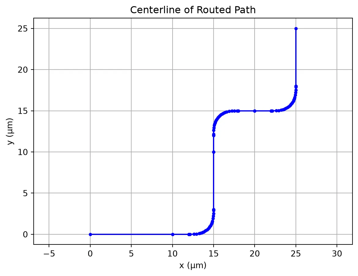
;fill:%23221f20;font-weight:bold;font-size:1.155000px;}.terminal{fill:none;stroke:%23805080;stroke-width:0.144375;}.dashed{stroke-dasharray:0.721875,0.433125;}.port{fill:none;stroke:%23805080;stroke-width:0.288750;}.virtual-connection{fill:none;stroke:%23907090;stroke-width:0.216563;}.layer_5_0{stroke:%23998573;fill:url(%23pat-layer_5_0);fill-opacity:0.492;}.label_5_0{fill:%23998573;}.layer_3_0{stroke:%238851ad;fill:url(%23pat-layer_3_0);fill-opacity:0.492;}.label_3_0{fill:%238851ad;}.layer_4_0{stroke:%23535e59;fill:url(%23pat-layer_4_0);fill-opacity:0.492;}.label_4_0{fill:%23535e59;}.layer_1_0{stroke:%23858d89;fill:url(%23pat-layer_1_0);fill-opacity:0.492;}.label_1_0{fill:%23858d89;}.layer_2_0{stroke:%235b98b9;fill:url(%23pat-layer_2_0);fill-opacity:0.492;}.label_2_0{fill:%235b98b9;}</style><defs><path id=%22port-symbol%22 class=%22port%22 d=%22M 0,-0.577500 L 0.866250,0 0,0.577500%22 /><path id=%22ref-port-symbol%22 class=%22port%22 style=%22stroke-opacity:0.33;%22 d=%22M 0,-0.433125 C 0.577500,-0.433125 0.577500,0.433125 0,0.433125%22 /><circle id=%22port-bend-symbol%22 style=%22stroke-width:0;stroke:none;fill:%23805080;fill-opacity:1;%22 cx=%220%22 cy=%220%22 r=%220.259875%22 /><circle id=%22connection-symbol%22 style=%22stroke-width:0;stroke:none;fill:%23907090;fill-opacity:1;%22 cx=%220%22 cy=%220%22 r=%220.303188%22 /><pattern id=%22pat-layer_5_0%22 patternUnits=%22userSpaceOnUse%22 width=%220.721875%22 height=%220.721875%22 patternTransform=%22translate(0.042463,0.645888)%22><line x1=%220.721875%22 y1=%220%22 x2=%220%22 y2=%220.721875%22 style=%22stroke:%23998573;stroke-width:0.072188%22 /><line x1=%221.082813%22 y1=%220.360938%22 x2=%220.360938%22 y2=%221.082813%22 style=%22stroke:%23998573;stroke-width:0.072188%22 /><line x1=%220.360938%22 y1=%22-0.360938%22 x2=%22-0.360938%22 y2=%220.360938%22 style=%22stroke:%23998573;stroke-width:0.072188%22 /></pattern><pattern id=%22pat-layer_3_0%22 patternUnits=%22userSpaceOnUse%22 width=%220.433125%22 height=%220.433125%22 patternTransform=%22translate(0.101912,0.319145)%22><circle cx=%220.216563%22 cy=%220.216563%22 r=%220.072188%22 style=%22stroke:none;fill:%238851ad;fill-opacity:1.0%22 /></pattern><pattern id=%22pat-layer_4_0%22 patternUnits=%22userSpaceOnUse%22 width=%220.721875%22 height=%220.721875%22 patternTransform=%22translate(0.467096,0.227961)%22><line x1=%220.360938%22 y1=%220%22 x2=%220.360938%22 y2=%220.721875%22 style=%22stroke:%23535e59;stroke-width:0.072188%22 /><line x1=%220%22 y1=%220.360938%22 x2=%220.721875%22 y2=%220.360938%22 style=%22stroke:%23535e59;stroke-width:0.072188%22 /></pattern><pattern id=%22pat-layer_1_0%22 patternUnits=%22userSpaceOnUse%22 width=%220.721875%22 height=%220.721875%22 patternTransform=%22translate(0.297243,0.417928)%22><circle cx=%220.360938%22 cy=%220.360938%22 r=%220.072188%22 style=%22stroke:none;fill:%23858d89;fill-opacity:1.0%22 /></pattern><pattern id=%22pat-layer_2_0%22 patternUnits=%22userSpaceOnUse%22 width=%220.721875%22 height=%220.721875%22 patternTransform=%22translate(0.594485,0.113980)%22><line x1=%220%22 y1=%220%22 x2=%220.721875%22 y2=%220.721875%22 style=%22stroke:%235b98b9;stroke-width:0.072188%22 /><line x1=%22-0.360938%22 y1=%220.360938%22 x2=%220.360938%22 y2=%221.082813%22 style=%22stroke:%235b98b9;stroke-width:0.072188%22 /><line x1=%220.360938%22 y1=%22-0.360938%22 x2=%221.082813%22 y2=%220.360938%22 style=%22stroke:%235b98b9;stroke-width:0.072188%22 /></pattern><g id=%22C1%22 data-name=%22straight__FOVXP6JOZ6YY6FSA6LNG3YTP6WXNZXBGXB5DHB6DS5RJG2NHTVOA%22><path class=%22layer_1_0%22 d=%22M 0.000000,-1.250000 10.000000,-1.250000 10.000000,1.250000 0.000000,1.250000 z%22 /><path class=%22layer_2_0%22 d=%22M 0.000000,-0.250000 10.000000,-0.250000 10.000000,0.250000 0.000000,0.250000 z%22 /></g><g id=%22C2%22 data-name=%22straight__WAWB6FWEXM52Y43SP5462XJMQ45RXQL32WH3JOKND3RU35R2Y7IA%22><path class=%22layer_1_0%22 d=%22M 0.000000,-1.250000 2.000000,-1.250000 2.000000,1.250000 0.000000,1.250000 z%22 /><path class=%22layer_2_0%22 d=%22M 0.000000,-0.250000 2.000000,-0.250000 2.000000,0.250000 0.000000,0.250000 z%22 /></g><g id=%22C3%22 data-name=%22bend__IJGSX32PNEZTIP44PO7Q5BDSAZNSMCCASSAEDYLKKCEYZIVH57KA%22><path class=%22layer_1_0%22 d=%22M 0.000000,-1.250000 0.693000,-1.237000 1.089000,-1.202000 1.299000,-1.171000 1.516000,-1.128000 1.738000,-1.071000 1.964000,-0.998000 2.193000,-0.907000 2.415000,-0.798000 2.630000,-0.673000 2.834000,-0.533000 3.028000,-0.378000 3.209000,-0.209000 3.378000,-0.028000 3.533000,0.166000 3.673000,0.370000 3.798000,0.585000 3.907000,0.807000 3.998000,1.036000 4.071000,1.262000 4.128000,1.484000 4.171000,1.701000 4.223000,2.113000 4.245000,2.493000 4.250000,3.000000 1.750000,3.000000 1.740000,2.445000 1.721000,2.221000 1.689000,2.032000 1.646000,1.882000 1.593000,1.763000 1.525000,1.655000 1.442000,1.558000 1.345000,1.475000 1.237000,1.407000 1.118000,1.354000 0.968000,1.311000 0.779000,1.279000 0.555000,1.260000 0.000000,1.250000 z%22 /><path class=%22layer_2_0%22 d=%22M 0.000000,-0.250000 0.637000,-0.238000 0.965000,-0.209000 1.296000,-0.152000 1.462000,-0.110000 1.626000,-0.057000 1.787000,0.007000 1.944000,0.084000 2.095000,0.172000 2.238000,0.270000 2.374000,0.379000 2.502000,0.498000 2.621000,0.626000 2.730000,0.762000 2.828000,0.905000 2.916000,1.056000 2.993000,1.213000 3.057000,1.374000 3.110000,1.538000 3.185000,1.869000 3.227000,2.199000 3.245000,2.524000 3.250000,3.000000 2.750000,3.000000 2.745000,2.540000 2.729000,2.242000 2.692000,1.953000 2.630000,1.676000 2.536000,1.415000 2.406000,1.173000 2.328000,1.059000 2.149000,0.851000 1.941000,0.672000 1.827000,0.594000 1.585000,0.464000 1.457000,0.413000 1.187000,0.335000 0.903000,0.287000 0.610000,0.261000 0.000000,0.250000 z%22 /></g><g id=%22C4%22 data-name=%22straight__AEXJR27OJYXRDZVLBGWPBNEMI374W4OOGLPRQQAKZTSUGNH72ADQ%22><path class=%22layer_1_0%22 d=%22M 0.000000,-1.250000 7.000000,-1.250000 7.000000,1.250000 0.000000,1.250000 z%22 /><path class=%22layer_2_0%22 d=%22M 0.000000,-0.250000 7.000000,-0.250000 7.000000,0.250000 0.000000,0.250000 z%22 /></g><g id=%22C5%22 data-name=%22bend__RFT52DMTWY3R3S346C24THXR5R5LCMBJSUQUGZIQOSG2BF2ZNQHA%22><path class=%22layer_1_0%22 d=%22M 0.000000,-1.250000 0.555000,-1.260000 0.779000,-1.279000 0.968000,-1.311000 1.118000,-1.354000 1.237000,-1.407000 1.345000,-1.475000 1.442000,-1.558000 1.525000,-1.655000 1.593000,-1.763000 1.646000,-1.882000 1.689000,-2.032000 1.721000,-2.221000 1.740000,-2.445000 1.750000,-3.000000 4.250000,-3.000000 4.245000,-2.493000 4.223000,-2.113000 4.171000,-1.701000 4.128000,-1.484000 4.071000,-1.262000 3.998000,-1.036000 3.907000,-0.807000 3.798000,-0.585000 3.673000,-0.370000 3.533000,-0.166000 3.378000,0.028000 3.209000,0.209000 3.028000,0.378000 2.834000,0.533000 2.630000,0.673000 2.415000,0.798000 2.193000,0.907000 1.964000,0.998000 1.738000,1.071000 1.516000,1.128000 1.299000,1.171000 1.089000,1.202000 0.693000,1.237000 0.000000,1.250000 z%22 /><path class=%22layer_2_0%22 d=%22M 0.000000,-0.250000 0.610000,-0.261000 0.903000,-0.287000 1.187000,-0.335000 1.457000,-0.413000 1.585000,-0.464000 1.827000,-0.594000 1.941000,-0.672000 2.149000,-0.851000 2.328000,-1.059000 2.406000,-1.173000 2.536000,-1.415000 2.630000,-1.676000 2.692000,-1.953000 2.729000,-2.242000 2.745000,-2.540000 2.750000,-3.000000 3.250000,-3.000000 3.245000,-2.524000 3.227000,-2.199000 3.185000,-1.869000 3.110000,-1.538000 3.057000,-1.374000 2.993000,-1.213000 2.916000,-1.056000 2.828000,-0.905000 2.730000,-0.762000 2.621000,-0.626000 2.502000,-0.498000 2.374000,-0.379000 2.238000,-0.270000 2.095000,-0.172000 1.944000,-0.084000 1.787000,-0.007000 1.626000,0.057000 1.462000,0.110000 1.296000,0.152000 0.965000,0.209000 0.637000,0.238000 0.000000,0.250000 z%22 /></g></defs><g transform=%22scale(1 -1)%22><g id=%22C0%22 data-name=%22RouteExample%22><use transform=%22translate(0.000000 0.000000)%22 href=%22%23C1%22 /><use transform=%22translate(10.000000 0.000000)%22 href=%22%23C2%22 /><use transform=%22translate(12.000000 0.000000)%22 href=%22%23C3%22 /><use transform=%22translate(15.000000 3.000000) rotate(90.000000)%22 href=%22%23C4%22 /><use transform=%22translate(15.000000 10.000000) rotate(90.000000)%22 href=%22%23C2%22 /><use transform=%22translate(15.000000 12.000000) rotate(90.000000)%22 href=%22%23C5%22 /><use transform=%22translate(18.000000 15.000000)%22 href=%22%23C2%22 /><use transform=%22translate(20.000000 15.000000)%22 href=%22%23C2%22 /><use transform=%22translate(22.000000 15.000000)%22 href=%22%23C3%22 /><use transform=%22translate(25.000000 18.000000) rotate(90.000000)%22 href=%22%23C4%22 /><g transform=%22translate(0.000000 0.000000) rotate(0.000000)%22><path class=%22port%22 d=%22M 0,-1.125000 V 1.125000%22 /><use href=%22%23port-symbol%22 /></g><text class=%22label%22 text-anchor=%22start%22 dominant-baseline=%22text-after-edge%22 x=%220.000000%22 y=%22-0.000000%22>P0</text><g transform=%22translate(25.000000 25.000000) rotate(270.000000)%22><path class=%22port%22 d=%22M 0,-1.125000 V 1.125000%22 /><use href=%22%23port-symbol%22 /></g><text class=%22label%22 text-anchor=%22start%22 dominant-baseline=%22text-before-edge%22 x=%2225.000000%22 y=%22-25.000000%22>P1</text></g></g></svg>)
Adding a Bulge to Straight Segments
Section titled “Adding a Bulge to Straight Segments”PhotonForge allows you to apply a bulge to straight segments in a routed path. This can be used to locally widen sections of the waveguide. The bulge_width sets the maximum width, bulge_taper_length controls how gradually the width transitions, and bulge_margin adjusts spacing around the bulge region.
route_example.update( straight_kwargs={"bulge_width": 0.6, "bulge_taper_length": 2, "bulge_margin": 0});fill:%23221f20;font-weight:bold;font-size:1.168200px;}.terminal{fill:none;stroke:%23805080;stroke-width:0.146025;}.dashed{stroke-dasharray:0.730125,0.438075;}.port{fill:none;stroke:%23805080;stroke-width:0.292050;}.virtual-connection{fill:none;stroke:%23907090;stroke-width:0.219038;}.layer_5_0{stroke:%23998573;fill:url(%23pat-layer_5_0);fill-opacity:0.492;}.label_5_0{fill:%23998573;}.layer_3_0{stroke:%238851ad;fill:url(%23pat-layer_3_0);fill-opacity:0.492;}.label_3_0{fill:%238851ad;}.layer_4_0{stroke:%23535e59;fill:url(%23pat-layer_4_0);fill-opacity:0.492;}.label_4_0{fill:%23535e59;}.layer_1_0{stroke:%23858d89;fill:url(%23pat-layer_1_0);fill-opacity:0.492;}.label_1_0{fill:%23858d89;}.layer_2_0{stroke:%235b98b9;fill:url(%23pat-layer_2_0);fill-opacity:0.492;}.label_2_0{fill:%235b98b9;}</style><defs><path id=%22port-symbol%22 class=%22port%22 d=%22M 0,-0.584100 L 0.876150,0 0,0.584100%22 /><path id=%22ref-port-symbol%22 class=%22port%22 style=%22stroke-opacity:0.33;%22 d=%22M 0,-0.438075 C 0.584100,-0.438075 0.584100,0.438075 0,0.438075%22 /><circle id=%22port-bend-symbol%22 style=%22stroke-width:0;stroke:none;fill:%23805080;fill-opacity:1;%22 cx=%220%22 cy=%220%22 r=%220.262845%22 /><circle id=%22connection-symbol%22 style=%22stroke-width:0;stroke:none;fill:%23907090;fill-opacity:1;%22 cx=%220%22 cy=%220%22 r=%220.306653%22 /><pattern id=%22pat-layer_5_0%22 patternUnits=%22userSpaceOnUse%22 width=%220.730125%22 height=%220.730125%22 patternTransform=%22translate(0.042949,0.653270)%22><line x1=%220.730125%22 y1=%220%22 x2=%220%22 y2=%220.730125%22 style=%22stroke:%23998573;stroke-width:0.073013%22 /><line x1=%221.095188%22 y1=%220.365063%22 x2=%220.365063%22 y2=%221.095188%22 style=%22stroke:%23998573;stroke-width:0.073013%22 /><line x1=%220.365063%22 y1=%22-0.365063%22 x2=%22-0.365063%22 y2=%220.365063%22 style=%22stroke:%23998573;stroke-width:0.073013%22 /></pattern><pattern id=%22pat-layer_3_0%22 patternUnits=%22userSpaceOnUse%22 width=%220.438075%22 height=%220.438075%22 patternTransform=%22translate(0.103076,0.322792)%22><circle cx=%220.219038%22 cy=%220.219038%22 r=%220.073013%22 style=%22stroke:none;fill:%238851ad;fill-opacity:1.0%22 /></pattern><pattern id=%22pat-layer_4_0%22 patternUnits=%22userSpaceOnUse%22 width=%220.730125%22 height=%220.730125%22 patternTransform=%22translate(0.472434,0.230566)%22><line x1=%220.365063%22 y1=%220%22 x2=%220.365063%22 y2=%220.730125%22 style=%22stroke:%23535e59;stroke-width:0.073013%22 /><line x1=%220%22 y1=%220.365063%22 x2=%220.730125%22 y2=%220.365063%22 style=%22stroke:%23535e59;stroke-width:0.073013%22 /></pattern><pattern id=%22pat-layer_1_0%22 patternUnits=%22userSpaceOnUse%22 width=%220.730125%22 height=%220.730125%22 patternTransform=%22translate(0.300640,0.422704)%22><circle cx=%220.365063%22 cy=%220.365063%22 r=%220.073013%22 style=%22stroke:none;fill:%23858d89;fill-opacity:1.0%22 /></pattern><pattern id=%22pat-layer_2_0%22 patternUnits=%22userSpaceOnUse%22 width=%220.730125%22 height=%220.730125%22 patternTransform=%22translate(0.601279,0.115283)%22><line x1=%220%22 y1=%220%22 x2=%220.730125%22 y2=%220.730125%22 style=%22stroke:%235b98b9;stroke-width:0.073013%22 /><line x1=%22-0.365063%22 y1=%220.365063%22 x2=%220.365063%22 y2=%221.095188%22 style=%22stroke:%235b98b9;stroke-width:0.073013%22 /><line x1=%220.365063%22 y1=%22-0.365063%22 x2=%221.095188%22 y2=%220.365063%22 style=%22stroke:%235b98b9;stroke-width:0.073013%22 /></pattern><g id=%22C1%22 data-name=%22straight__DJM37JL3BJST62FCIY6HXYTSGPVAT5GLRDRD7B5MMS4OLO2PPH5Q%22><path class=%22layer_1_0%22 d=%22M 0.000000,-1.250000 1.000000,-1.400000 2.000000,-1.550000 8.000000,-1.550000 9.000000,-1.400000 10.000000,-1.250000 10.000000,1.250000 9.000000,1.400000 8.000000,1.550000 2.000000,1.550000 1.000000,1.400000 0.000000,1.250000 z%22 /><path class=%22layer_2_0%22 d=%22M 0.000000,-0.250000 1.000000,-0.400000 2.000000,-0.550000 8.000000,-0.550000 9.000000,-0.400000 10.000000,-0.250000 10.000000,0.250000 9.000000,0.400000 8.000000,0.550000 2.000000,0.550000 1.000000,0.400000 0.000000,0.250000 z%22 /></g><g id=%22C2%22 data-name=%22straight__4GZF23SYMUOADVVOA4EFYWUPP2J6MUUL6MNKJCNQR7OM5AD7JEDQ%22><path class=%22layer_1_0%22 d=%22M 0.000000,-1.250000 2.000000,-1.250000 2.000000,1.250000 0.000000,1.250000 z%22 /><path class=%22layer_2_0%22 d=%22M 0.000000,-0.250000 2.000000,-0.250000 2.000000,0.250000 0.000000,0.250000 z%22 /></g><g id=%22C3%22 data-name=%22bend__IJGSX32PNEZTIP44PO7Q5BDSAZNSMCCASSAEDYLKKCEYZIVH57KA%22><path class=%22layer_1_0%22 d=%22M 0.000000,-1.250000 0.693000,-1.237000 1.089000,-1.202000 1.299000,-1.171000 1.516000,-1.128000 1.738000,-1.071000 1.964000,-0.998000 2.193000,-0.907000 2.415000,-0.798000 2.630000,-0.673000 2.834000,-0.533000 3.028000,-0.378000 3.209000,-0.209000 3.378000,-0.028000 3.533000,0.166000 3.673000,0.370000 3.798000,0.585000 3.907000,0.807000 3.998000,1.036000 4.071000,1.262000 4.128000,1.484000 4.171000,1.701000 4.223000,2.113000 4.245000,2.493000 4.250000,3.000000 1.750000,3.000000 1.740000,2.445000 1.721000,2.221000 1.689000,2.032000 1.646000,1.882000 1.593000,1.763000 1.525000,1.655000 1.442000,1.558000 1.345000,1.475000 1.237000,1.407000 1.118000,1.354000 0.968000,1.311000 0.779000,1.279000 0.555000,1.260000 0.000000,1.250000 z%22 /><path class=%22layer_2_0%22 d=%22M 0.000000,-0.250000 0.637000,-0.238000 0.965000,-0.209000 1.296000,-0.152000 1.462000,-0.110000 1.626000,-0.057000 1.787000,0.007000 1.944000,0.084000 2.095000,0.172000 2.238000,0.270000 2.374000,0.379000 2.502000,0.498000 2.621000,0.626000 2.730000,0.762000 2.828000,0.905000 2.916000,1.056000 2.993000,1.213000 3.057000,1.374000 3.110000,1.538000 3.185000,1.869000 3.227000,2.199000 3.245000,2.524000 3.250000,3.000000 2.750000,3.000000 2.745000,2.540000 2.729000,2.242000 2.692000,1.953000 2.630000,1.676000 2.536000,1.415000 2.406000,1.173000 2.328000,1.059000 2.149000,0.851000 1.941000,0.672000 1.827000,0.594000 1.585000,0.464000 1.457000,0.413000 1.187000,0.335000 0.903000,0.287000 0.610000,0.261000 0.000000,0.250000 z%22 /></g><g id=%22C4%22 data-name=%22straight__ETHSKDNJZ7TSJ3AKCY2HUQM6SZB24LC3E5PCU2QQEHZRGCHEFWKQ%22><path class=%22layer_1_0%22 d=%22M 0.000000,-1.250000 1.000000,-1.400000 2.000000,-1.550000 5.000000,-1.550000 6.000000,-1.400000 7.000000,-1.250000 7.000000,1.250000 6.000000,1.400000 5.000000,1.550000 2.000000,1.550000 1.000000,1.400000 0.000000,1.250000 z%22 /><path class=%22layer_2_0%22 d=%22M 0.000000,-0.250000 1.000000,-0.400000 2.000000,-0.550000 5.000000,-0.550000 6.000000,-0.400000 7.000000,-0.250000 7.000000,0.250000 6.000000,0.400000 5.000000,0.550000 2.000000,0.550000 1.000000,0.400000 0.000000,0.250000 z%22 /></g><g id=%22C5%22 data-name=%22bend__RFT52DMTWY3R3S346C24THXR5R5LCMBJSUQUGZIQOSG2BF2ZNQHA%22><path class=%22layer_1_0%22 d=%22M 0.000000,-1.250000 0.555000,-1.260000 0.779000,-1.279000 0.968000,-1.311000 1.118000,-1.354000 1.237000,-1.407000 1.345000,-1.475000 1.442000,-1.558000 1.525000,-1.655000 1.593000,-1.763000 1.646000,-1.882000 1.689000,-2.032000 1.721000,-2.221000 1.740000,-2.445000 1.750000,-3.000000 4.250000,-3.000000 4.245000,-2.493000 4.223000,-2.113000 4.171000,-1.701000 4.128000,-1.484000 4.071000,-1.262000 3.998000,-1.036000 3.907000,-0.807000 3.798000,-0.585000 3.673000,-0.370000 3.533000,-0.166000 3.378000,0.028000 3.209000,0.209000 3.028000,0.378000 2.834000,0.533000 2.630000,0.673000 2.415000,0.798000 2.193000,0.907000 1.964000,0.998000 1.738000,1.071000 1.516000,1.128000 1.299000,1.171000 1.089000,1.202000 0.693000,1.237000 0.000000,1.250000 z%22 /><path class=%22layer_2_0%22 d=%22M 0.000000,-0.250000 0.610000,-0.261000 0.903000,-0.287000 1.187000,-0.335000 1.457000,-0.413000 1.585000,-0.464000 1.827000,-0.594000 1.941000,-0.672000 2.149000,-0.851000 2.328000,-1.059000 2.406000,-1.173000 2.536000,-1.415000 2.630000,-1.676000 2.692000,-1.953000 2.729000,-2.242000 2.745000,-2.540000 2.750000,-3.000000 3.250000,-3.000000 3.245000,-2.524000 3.227000,-2.199000 3.185000,-1.869000 3.110000,-1.538000 3.057000,-1.374000 2.993000,-1.213000 2.916000,-1.056000 2.828000,-0.905000 2.730000,-0.762000 2.621000,-0.626000 2.502000,-0.498000 2.374000,-0.379000 2.238000,-0.270000 2.095000,-0.172000 1.944000,-0.084000 1.787000,-0.007000 1.626000,0.057000 1.462000,0.110000 1.296000,0.152000 0.965000,0.209000 0.637000,0.238000 0.000000,0.250000 z%22 /></g></defs><g transform=%22scale(1 -1)%22><g id=%22C0%22 data-name=%22RouteExample%22><use transform=%22translate(0.000000 0.000000)%22 href=%22%23C1%22 /><use transform=%22translate(10.000000 0.000000)%22 href=%22%23C2%22 /><use transform=%22translate(12.000000 0.000000)%22 href=%22%23C3%22 /><use transform=%22translate(15.000000 3.000000) rotate(90.000000)%22 href=%22%23C4%22 /><use transform=%22translate(15.000000 10.000000) rotate(90.000000)%22 href=%22%23C2%22 /><use transform=%22translate(15.000000 12.000000) rotate(90.000000)%22 href=%22%23C5%22 /><use transform=%22translate(18.000000 15.000000)%22 href=%22%23C2%22 /><use transform=%22translate(20.000000 15.000000)%22 href=%22%23C2%22 /><use transform=%22translate(22.000000 15.000000)%22 href=%22%23C3%22 /><use transform=%22translate(25.000000 18.000000) rotate(90.000000)%22 href=%22%23C4%22 /><g transform=%22translate(0.000000 0.000000) rotate(0.000000)%22><path class=%22port%22 d=%22M 0,-1.125000 V 1.125000%22 /><use href=%22%23port-symbol%22 /></g><text class=%22label%22 text-anchor=%22start%22 dominant-baseline=%22text-after-edge%22 x=%220.000000%22 y=%22-0.000000%22>P0</text><g transform=%22translate(25.000000 25.000000) rotate(270.000000)%22><path class=%22port%22 d=%22M 0,-1.125000 V 1.125000%22 /><use href=%22%23port-symbol%22 /></g><text class=%22label%22 text-anchor=%22start%22 dominant-baseline=%22text-before-edge%22 x=%2225.000000%22 y=%22-25.000000%22>P1</text></g></g></svg>)
Cladding Around a Path
Section titled “Cladding Around a Path”We create a path with two turns and then compute its offset boundary using offset(). We enable round_joins to round the corners. Finally, we add the offset polygons to the SLAB layer and the original path to the WG_CORE layer.
# Create a pathp = (    pf.Path((0, 0), width=0.5)  # Start at origin with width 0.5    .turn(45, radius=3)  # Turn 45° clockwise with radius 3    .segment((3, 3), relative=True)  # Move diagonally from current position    .turn(-45, radius=3)  # Turn 45° counter-clockwise with radius 3    .segment((5, 0), relative=True)  # Move horizontally to the right)
# Compute offset polygons around the path with distance 0.5 and rounded joinsenv_polygons = pf.offset(p, distance=0.5, round_joins=True)
# Create a component to hold the path and its offset boundaryc = pf.Component()
# Add each offset polygon to the "SLAB" layerc.add("SLAB", *env_polygons)
# Add the original path to the "WG_CORE" layerc.add("WG_CORE", p)
# Display the component with offset boundary and pathc