800G Coherent Receiver Components

Download notebook (.zip)

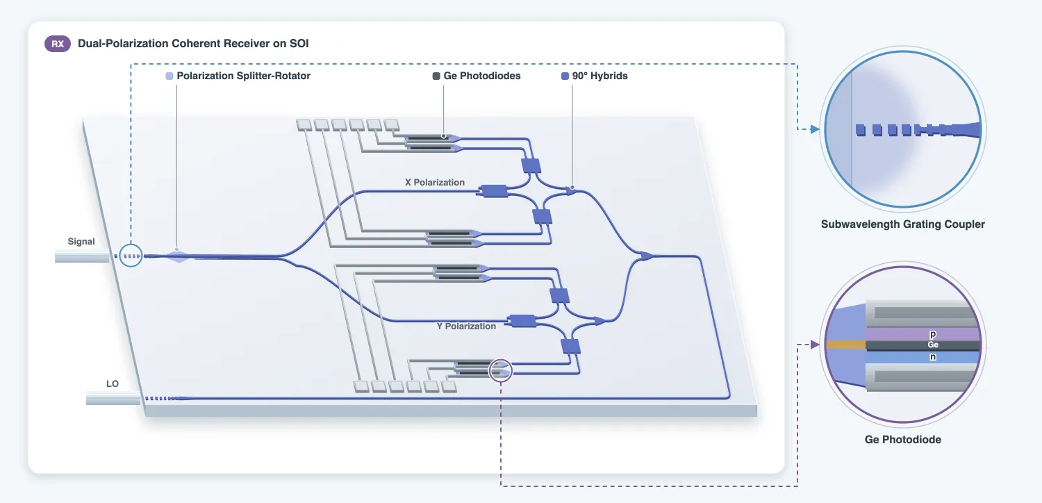
This page designs the components of the receiver chip on the SOI technology written on the technology page: the edge coupler that takes both polarizations from the fiber, the polarization splitter-rotator (PSR) that separates them, the 90 degree hybrid that mixes each polarization with the local oscillator (LO), and the germanium photodiode with its transimpedance amplifier (TIA). Each component gets a model, which the link page uses.

References

1. Cheben, Pavel, et al. “Broadband polarization independent nanophotonic coupler for silicon waveguides with ultra-high efficiency.” Optics Express 2015 23 (17), 22553-22563, doi: 10.1364/OE.23.022553.
2. Sacher, Wesley D., et al. “Polarization rotator-splitters in standard active silicon photonics platforms.” Optics Express 2014 22 (4), 3777-3786, doi: 10.1364/OE.22.003777.
3. Guan, Hang, et al. “Compact and low loss 90 degree optical hybrid on a silicon-on-insulator platform.” Optics Express 2017 25 (23), 28957-28968, doi: 10.1364/OE.25.028957.
4. Chen, Hongtao, et al. “-1 V bias 67 GHz bandwidth Si-contacted germanium waveguide p-i-n photodetector for optical links at 56 Gbps and beyond.” Optics Express 2016 24 (5), 4622-4631, doi: 10.1364/OE.24.004622.
5. Gläsel, Jonas, et al. “128 GBaud coherent receiver engine with flat frequency response.” Optical Fiber Communication Conference (OFC) 2024, paper W1K.7.

The longer simulations of this page are loaded from three data files: coherent_rx_taper_profile.json, coherent_rx_edge_coupler.json and coherent_rx_psr.json. Each is followed by a commented cell with the code that produces it, which can be uncommented to run the simulation again or to try a different structure.

from runpy import run_path

# Coherent_Technology.qmd defines what this page builds on. Its shared cells are generated into the
# module below; see docs/scripts/generate_notebook_modules.py.
globals().update(
    {k: v for k, v in run_path("misc/coherent_technology.py").items() if not k.startswith("_")}
)

import json

import photonforge.abstract as pfa
import tidy3d.web as web

pf.config.default_technology = tech_rx
viewer = pf.live_viewer.LiveViewer()

LiveViewer started at http://127.0.0.1:36873. Call its 'stop()' method to free the port.

Edge coupler

The signal arrives in a standard single-mode fiber in an arbitrary polarization, so the receiver edge coupler has to couple TE and TM with similar loss. A silicon wire tapered to a narrow tip does this poorly, because the TM mode of a narrow wire is cut off well before the TE mode. The coupler here is a subwavelength grating (SWG) after Cheben et al. [1]: silicon segments shorter than the wavelength act as a uniform medium of intermediate index, and the expanded mode of that medium couples to the fiber in both polarizations.

The coupler has three sections:

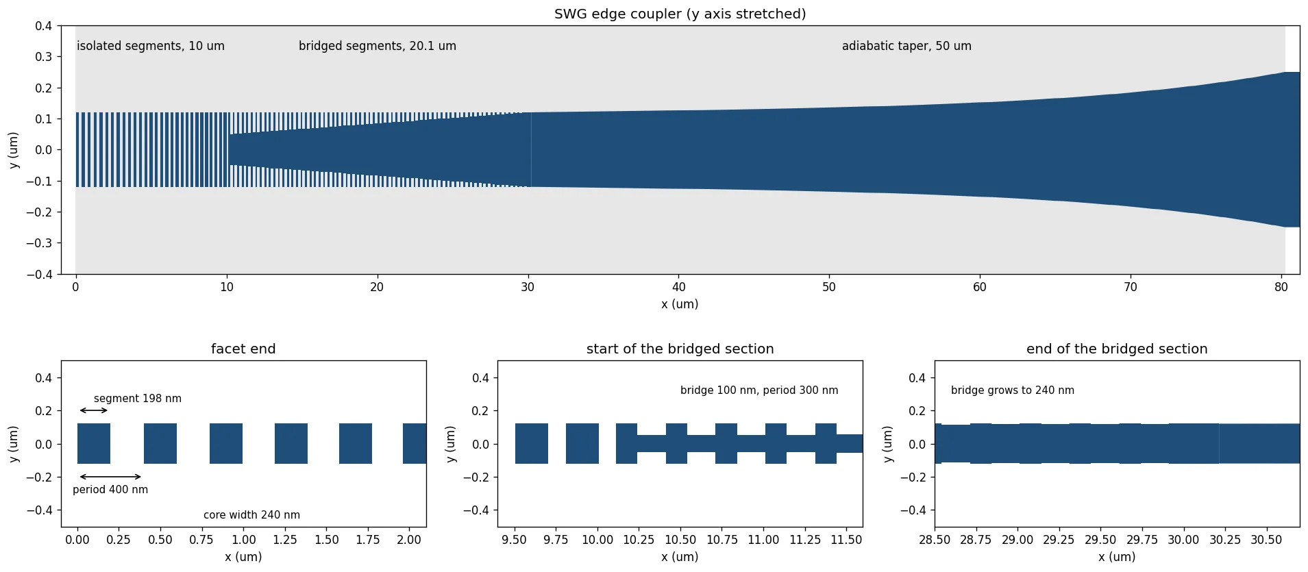
• Isolated segments, 10 um long, whose period shrinks from 400 to 300 nm. At the facet the segments are sparse and the mode is large; the shrinking period raises the average index and pulls the mode in.
• Bridged segments, 67 periods of 300 nm, joined by a bridge whose width grows from 100 nm to the 240 nm of the wire. The SWG mode turns into the mode of a solid wire without a jump in index.
• Adiabatic taper from 240 to 500 nm over 50 um, with a width profile that keeps the mode conversion loss constant along it. The profile was computed from the mode solutions of the wire at each width and is loaded from coherent_rx_taper_profile.json.

The fiber is a high numerical aperture fiber (UHNA7, numerical aperture 0.41, 2.4 um core) with a mode field diameter of 3.2 um, spliced to the standard fiber of the link. It is modelled as a FiberPort with a slightly elliptical core, which separates its two polarization modes so the port can tell them apart. Every line and space of the drawing is 100 nm or larger.

The drawing below shows the coupler to scale, in the style of the figures of Cheben et al. [1]. At the facet the segments are 198 nm long on a 400 nm period, so only half of each period is silicon and the effective index of the core is low: the mode spreads far into the cladding and matches the fiber. Along the isolated section the period shrinks to 300 nm, which raises the effective index and pulls the mode in. In the bridged section a thin bridge between the segments grows from 100 nm to the full 240 nm width, until the core is a solid wire; the bridge raises the index gradually, so the mode never meets a step. The adiabatic taper then widens the wire to the 500 nm strip of the chip.

w_tip = 0.24  # SWG core width (um)
l_isolated = 10.0  # Isolated section length (um)
# Isolated-section period at the facet and at its end (um)
pitch_start, pitch_end = 0.400, 0.300
# Isolated-section segment length at the facet and at its end (um)
seg_start, seg_end = 0.198, 0.200
n_bridged = 67  # Periods in the bridged section
bridge_min = 0.100  # Narrowest bridge, the minimum feature size (um)
# Bridged-section segment length that keeps the average silicon fraction of the last isolated period
seg_bridged = (seg_end * w_tip - pitch_end * bridge_min) / (w_tip - bridge_min)
profile = json.load(open("misc/coherent_rx_taper_profile.json"))

# UHNA7 fiber: the cladding is silica, and the core index follows from the numerical aperture
n_clad = float(np.sqrt(sio2["optical"].eps_model(f0).real))
n_core = float(np.sqrt(n_clad**2 + 0.41**2))

@pf.parametric_component(name_prefix="EC_SWG_RX")
def swg_edge_coupler(*, model=None):
    c = pf.Component()

    # Isolated segments, period and segment length ramped linearly
    x = 0.0
    while x < l_isolated:
        t = x / l_isolated
        pitch = pitch_start + (pitch_end - pitch_start) * t
        seg = seg_start + (seg_end - seg_start) * t
        c.add("Si", pf.Rectangle((x, -w_tip / 2), (x + seg, w_tip / 2)))
        x += pitch

    # Bridged segments: full-width segment plus a bridge growing to the wire width
    for i in range(n_bridged):
        w_bridge = bridge_min + (w_tip - bridge_min) * i / (n_bridged - 1)
        c.add(
            "Si",
            pf.Rectangle((x, -w_tip / 2), (x + seg_bridged, w_tip / 2)),
            pf.Rectangle(
                (x + seg_bridged, -w_bridge / 2), (x + pitch_end, w_bridge / 2)
            ),
        )
        x += pitch_end

    # Adiabatic taper to the 500 nm wire, then 1 um of wire
    xs = x + np.array(profile["xf"])[::4]
    ws = np.array(profile["wf"])[::4]
    x_end = xs[-1] + 1.0
    upper = [(a, b / 2) for a, b in zip(xs, ws)] + [(x_end, 0.25)]
    c.add("Si", pf.Polygon(upper + [(a, -b) for a, b in upper[::-1]]))

    # The deep trench in front of the facet, where the fiber sits
    c.add("Deep Trench", pf.Rectangle((-20, -10), (0, 10)))

    # The fiber butted 1 um from the facet. Mode 0 is polarized along z (TM), mode 1 along y (TE).
    fiber = pf.FiberPort(
        center=(-1.0, 0, 0.11),
        input_vector=(1, 0, 0),
        size=(7.6, 6.6),
        extrusion_limits=(-50, 1.0),
        cross_section=[
            (pf.Circle(62.5), td.Medium(permittivity=n_clad**2)),
            # 1 % ellipticity separates the two polarization modes
            (pf.Circle((1.2 * 1.01, 1.2)), td.Medium(permittivity=n_core**2)),
        ],
        num_modes=2,
        target_neff=n_core,
    )
    c.add_port(fiber, "P0")
    c.add_port(pf.Port((x_end, 0), 180, "Strip_TE_TM"), "P1")
    if model is not None:
        c.add_model(model, "FDTD data")
    return c

ec_swg = swg_edge_coupler()
print(
    f"coupler length {ec_swg.ports['P1'].center[0]:.1f} um, bridged segment {seg_bridged * 1e3:.0f} nm"
)
viewer(ec_swg)

coupler length 81.2 um, bridged segment 129 nm

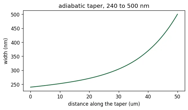
The taper is slowest where the wire is narrow and the mode is weakly guided, because that is where a fast change of width would scatter light. The profile follows from a condition on the local taper angle: it is held at a fixed fraction of $w / (2 z_b)$, with $z_b = \lambda / (n_\text{eff} - n_\text{clad})$ the beat length between the strip mode and the cladding. Since $\mathrm{d}w/\mathrm{d}x \propto w\,(n_\text{eff} - n_\text{clad})$, the profile is the integral of its inverse over the width, scaled to the chosen length of 50 um. The width along the taper is drawn below; the commented cell after it computes the profile from mode solutions of the strip at 15 widths.

# # Strip TE0 index against width, from 240 to 500 nm
# widths = np.round(np.linspace(0.24, 0.50, 15), 3)
# specs = [
#     pf.PortSpec(f"strip {w * 1e3:.0f} nm", width=3.0, limits=(-1.0, 1.22), num_modes=1, target_neff=3.5,
#                 path_profiles=[(w, 0, (1, 0))])
#     for w in widths
# ]
# solvers = pf.port_modes(specs, [f0], technology=tech_rx, mesh_refinement=40, verbose=False)
# n_eff_w = np.array([float(np.real(m.data.n_eff.values.ravel()[0])) for m in solvers])
# n_clad = float(np.sqrt(sio2["optical"].eps_model(f0).real))
# # Constant fraction of the local angle limit: dx/dw = 1 / (w (n_eff - n_clad)), integrated and scaled
# from scipy.interpolate import PchipInterpolator
# w_fine = np.linspace(widths[0], widths[-1], 281)
# dx_dw = 1.0 / (w_fine * (PchipInterpolator(widths, n_eff_w)(w_fine) - n_clad))
# x_fine = np.concatenate([[0], np.cumsum(0.5 * (dx_dw[1:] + dx_dw[:-1]) * np.diff(w_fine))])
# x_fine *= 50.0 / x_fine[-1]  # 50 um long
# with open("misc/coherent_rx_taper_profile.json", "w") as file:
#     json.dump(dict(width=widths.tolist(), n_eff=n_eff_w.tolist(), L=50.0, wf=w_fine.tolist(), xf=x_fine.tolist()), file)

The coupler is too long for one FDTD simulation at the mesh its 100 nm features need, so it was simulated in two parts with PML boundaries: the fiber, facet and SWG sections up to the 240 nm wire, and the adiabatic taper from 240 to 500 nm. The first part was run in reverse, from the wire mode to the fiber mode, which measures the overlap with the fiber mode directly. The product of the two complex transmissions is the coupler, for each polarization. The amplitudes are loaded from coherent_rx_edge_coupler.json into a DataModel. Reflections stay below $-25$ dB and the conversion between polarizations is zero by symmetry, so the model keeps only the two through paths.

ec_swg_data = json.load(open("misc/coherent_rx_edge_coupler.json"))
f_ec = np.array(ec_swg_data["TE"]["f"])
elements = {}
# Fiber mode 1 (polarized along y) couples to TE, fiber mode 0 (along z) to TM
for pol, fiber_mode, wire_mode in (("TE", "P0@1", "P1@0"), ("TM", "P0@0", "P1@1")):
    amp = np.array(ec_swg_data[pol]["re"]) + 1j * np.array(ec_swg_data[pol]["im"])
    elements[(fiber_mode, wire_mode)] = amp
    elements[(wire_mode, fiber_mode)] = amp
ec_swg_model = pf.DataModel(
    s_matrix=pf.SMatrix(f_ec, elements), interpolation_method="pchip"
)
ec_swg = swg_edge_coupler(model=ec_swg_model)

wl_plot = np.linspace(1.48, 1.58, 51)
s_ec_swg = ec_swg.s_matrix(pf.C_0 / wl_plot)
fig, ax = plt.subplots(1, 1, figsize=(6, 4))
for pol, key in (("TE", ("P0@1", "P1@0")), ("TM", ("P0@0", "P1@1"))):
    loss = -20 * np.log10(np.abs(s_ec_swg[key]))
    ax.plot(wl_plot * 1e3, loss, label=pol)
    print(f"{pol}: {np.interp(lda0, wl_plot, loss):.2f} dB at 1550 nm")
ax.set_xlabel("wavelength (nm)")
ax.set_ylabel("coupling loss (dB)")
ax.set_ylim(0, 1)
ax.legend()
plt.show()

TE: 0.41 dB at 1550 nm
TM: 0.61 dB at 1550 nm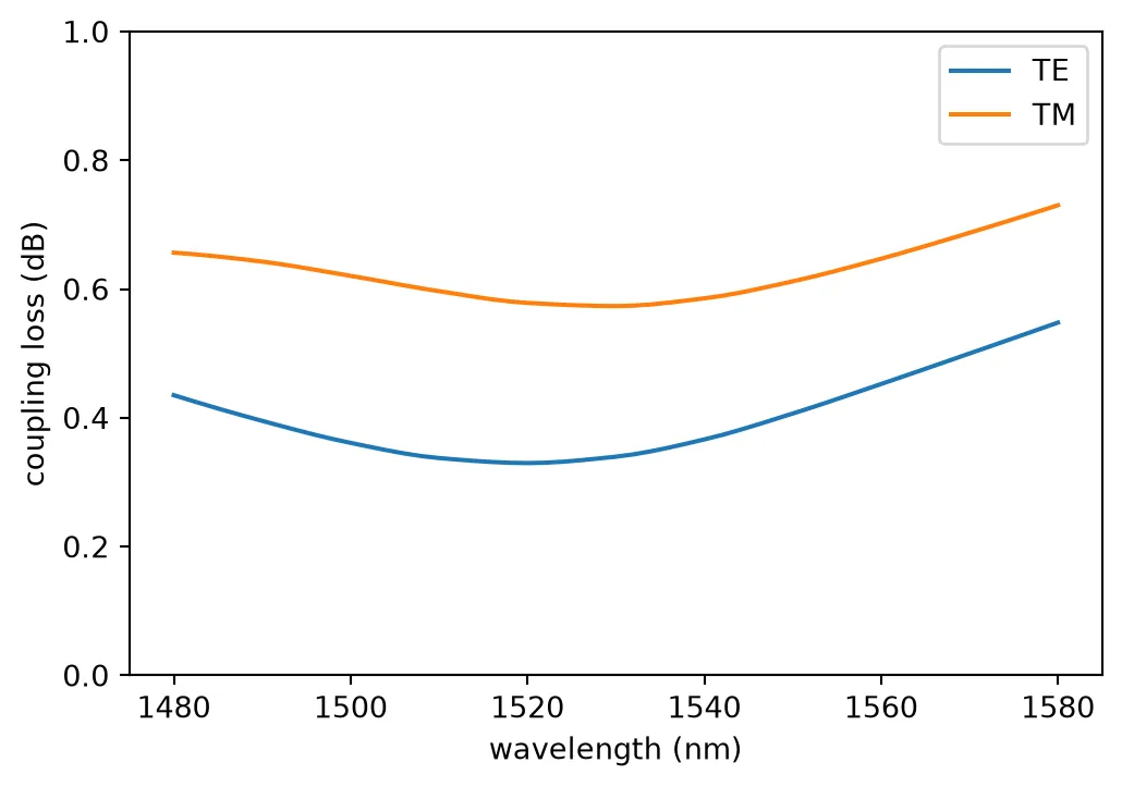

The commented cell below simulates the coupler with FDTD and writes the amplitudes in the format of the data file. It runs the whole coupler in one simulation per polarization, from the 500 nm strip to the fiber mode, which is simpler than the two parts the file was computed from. It uses the same mesh: 12 cells per wavelength, refined to 20 nm over the segments, which are 100 to 200 nm long.

# # One FDTD per polarization: the mirror plane at y = 0 selects TE (antisymmetric) or TM (symmetric)
# x_swg = l_isolated + n_bridged * pitch_end
# swg_mesh = td.GridSpec.auto(
#     min_steps_per_wvl=12,
#     wavelength=lda0,
#     override_structures=[
#         td.MeshOverrideStructure(geometry=td.Box.from_bounds((0, -0.15, 0), (x_swg, 0.15, 0.22)), dl=(0.02, 0.02, 0.02))
#     ],
# )
# wl_fdtd = np.linspace(1.48, 1.58, 11)
# result = {}
# for pol, sym, wire_mode, fiber_mode in (("TE", -1, "P1@0", "P0@1"), ("TM", 1, "P1@1", "P0@0")):
#     run = swg_edge_coupler(
#         model=pf.Tidy3DModel(
#             grid_spec=swg_mesh,
#             symmetry=(0, sym, 0),
#             boundary_spec=td.BoundarySpec.all_sides(td.PML()),
#             bounds=((-2.2, -4.0, -3.6), (None, 4.0, 3.6)),
#             verbose=False,
#         )
#     )
#     s = run.s_matrix(pf.C_0 / wl_fdtd, model_kwargs={"inputs": [wire_mode]})
#     amp = s[(wire_mode, fiber_mode)]
#     order = np.argsort(pf.C_0 / wl_fdtd)
#     result[pol] = dict(f=(pf.C_0 / wl_fdtd)[order].tolist(), re=amp[order].real.tolist(), im=amp[order].imag.tolist())
# with open("misc/coherent_rx_edge_coupler.json", "w") as file:
#     json.dump(result, file)

TE couples with about 0.4 dB and TM with about 0.6 dB, so the polarization-dependent loss of the coupler is about 0.2 dB. TM loses more because its mode is more confined vertically than the circular fiber mode, while the SWG expands the TE mode further. The DSP at the end of the link equalizes the two polarizations, and the link page includes this difference.

Polarization splitter-rotator

The PSR sends TE0 of its input to one output and converts TM0 into TE0 of a second output, so everything after it works in TE. It is the design of Sacher et al. [2], made of two sections that use only the full and partial silicon etches:

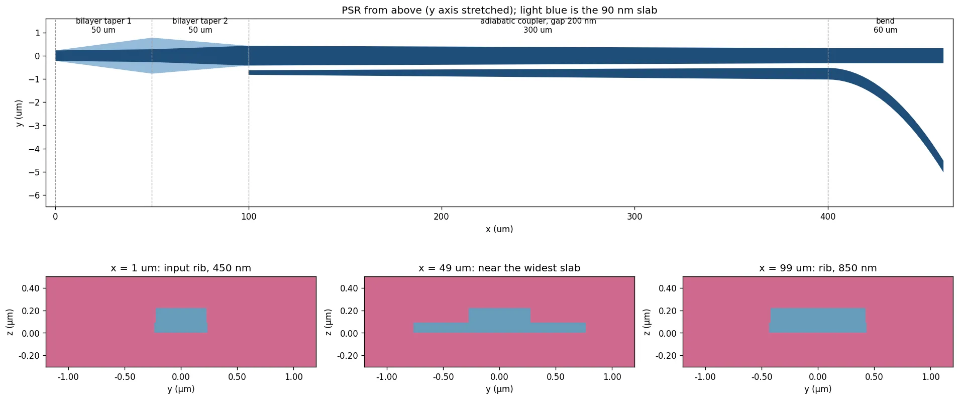
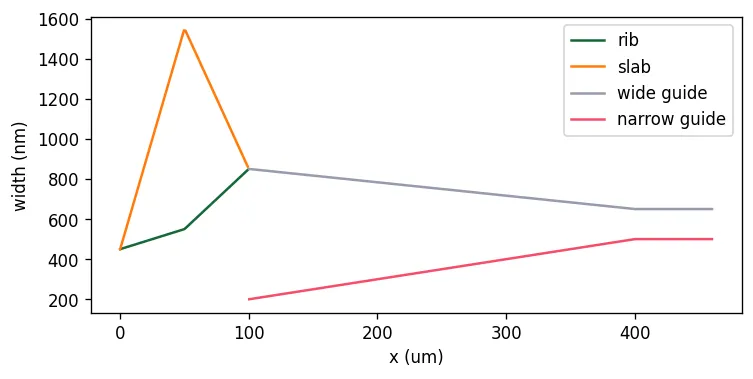
• A bilayer taper widens a rib from 450 to 850 nm while its 90 nm slab first widens and then narrows back. The slab breaks the vertical symmetry of the waveguide, and in that asymmetric cross-section TM0 and TE1 hybridize where their indices cross: an adiabatic taper through the crossing turns TM0 into TE1. TE0 is unaffected.
• An adiabatic coupler then moves TE1 of the wide guide into TE0 of a narrow guide beside it, which widens from 200 to 500 nm along 300 um at a 200 nm gap, and bends away.

The drawing below shows the PSR to scale in the style of Sacher et al. [2]. From above, the slab of the bilayer taper is the light diamond around the rib: it widens over the first 50 um and is absorbed back into the rib over the next 50 um. The three cuts across it show why it rotates the polarization. At the input the rib is a symmetric strip, where TM0 and TE1 cannot couple. In the middle the slab extends on both sides of the rib at its bottom only, so the cross-section is no longer symmetric top to bottom, and the two modes mix where their indices cross. At the end the slab has gone and TM0 has become TE1 of the 850 nm rib. In the coupler that follows, the wide guide narrows while the narrow guide widens, and TE1 of the wide guide passes into TE0 of the narrow one where their indices cross.

# Sacher PSR dimensions (um)
psr_dims = dict(
    rib_in=0.45,  # Input rib width
    rib_mid=0.55,  # Rib width at the end of the first taper
    rib_out=0.85,  # Rib width at the end of the bilayer taper
    fin_mid=0.5,  # Slab extension on each side at the end of the first taper
    la=50.0,  # First taper length
    lb=50.0,  # Second taper length
    broad_end=0.65,  # Wide guide at the end of the coupler
    narrow_start=0.2,  # Narrow guide at the start of the coupler
    narrow_end=0.5,  # Narrow guide at the end of the coupler
    gap=0.2,  # Coupler gap
    lc=300.0,  # Coupler length
    radius=450.0,  # Radius of the arc that takes the narrow guide away
    ld=60.0,  # Length of that arc section
)

@pf.parametric_component(name_prefix="PSR")
def psr(*, dims=psr_dims, model=None):
    d = dims
    c = pf.Component()
    xa = d["la"]
    xb = xa + d["lb"]
    xc = xb + d["lc"]
    xd = xc + d["ld"]

    # Bilayer taper: the full-height rib and the slab under it
    rib = [(0, d["rib_in"]), (xa, d["rib_mid"]), (xb, d["rib_out"])]
    slab = [(0, d["rib_in"]), (xa, d["rib_mid"] + 2 * d["fin_mid"]), (xb, d["rib_out"])]
    for layer, prof in (("Si", rib), ("Si Slab", slab)):
        top = [(x, w / 2) for x, w in prof]
        c.add(layer, pf.Polygon(top + [(x, -y) for x, y in top[::-1]]))

    # Adiabatic coupler: the wide guide narrows while the narrow guide beside it widens
    xs = np.linspace(xb, xd, 121)
    wb = np.interp(xs, [xb, xc, xd], [d["rib_out"], d["broad_end"], d["broad_end"]])
    c.add(
        "Si",
        pf.Polygon(
            [(x, w / 2) for x, w in zip(xs, wb)]
            + [(x, -w / 2) for x, w in zip(xs[::-1], wb[::-1])]
        ),
    )
    wn = np.interp(
        xs, [xb, xc, xd], [d["narrow_start"], d["narrow_end"], d["narrow_end"]]
    )
    drop = np.where(xs > xc, (xs - xc) ** 2 / (2 * d["radius"]), 0.0)
    inner = -(wb / 2 + d["gap"] + drop)
    c.add(
        "Si",
        pf.Polygon(
            [(x, y) for x, y in zip(xs, inner)]
            + [(x, y - w) for x, y, w in zip(xs[::-1], inner[::-1], wn[::-1])]
        ),
    )

    # P0: TE0 and TM0 in; P1: the wide guide (TE); P2: the narrow guide (rotated TM)
    y_narrow = inner[-1] - wn[-1] / 2
    two = pf.PortSpec(
        "PSR input",
        width=3.0,
        limits=(-1.0, 1.22),
        num_modes=2,
        target_neff=3.5,
        path_profiles=[(d["rib_in"], 0, (1, 0))],
    )
    broad = pf.PortSpec(
        "PSR wide arm",
        width=3.0,
        limits=(-1.0, 1.22),
        num_modes=1,
        target_neff=3.5,
        path_profiles=[(d["broad_end"], 0, (1, 0))],
    )
    narrow = pf.PortSpec(
        "PSR narrow arm",
        width=3.0,
        limits=(-1.0, 1.22),
        num_modes=1,
        target_neff=3.5,
        path_profiles=[(d["narrow_end"], 0, (1, 0))],
    )
    c.add_port(pf.Port((0, 0), 0, two), "P0")
    c.add_port(pf.Port((xd, 0), 180, broad), "P1")
    c.add_port(pf.Port((xd, y_narrow), 180, narrow), "P2")
    if model is not None:
        c.add_model(model, "data")
    return c

viewer(psr())

The two paths were solved separately. The TE path was converged by eigenmode expansion (EME): TE0 passes with no measurable loss and leaks below $-52$ dB into the narrow arm. The TM path depends on the mode hybridization in the bilayer taper and on the 200 nm gap, so it was simulated with 3D FDTD at 10 cells per wavelength with 20 nm cells across the gap. Its two amplitudes, TM0 to the narrow arm and TM0 leaking into the wide arm, are loaded from coherent_rx_psr.json with the group delay of the device, and become a PolarizationSplitterRotatorModel.

psr_data = json.load(open("misc/coherent_rx_psr.json"))
wl_psr = np.array(psr_data["wl"])
tau_psr = psr_data["tau_ps"] * 1e-12  # Group delay of the device (s)

# Each path is its magnitude times the device delay, sampled densely so the delay phase interpolates
f_model = pf.C_0 / np.linspace(1.45, 1.65, 6001)
magnitude = lambda m: np.interp(f_model, pf.C_0 / wl_psr[::-1], np.array(m)[::-1])
path = lambda m: pf.Interpolator(
    f_model, m * np.exp(2j * np.pi * (f_model - f0) * tau_psr), coords="mag_phase"
)
psr_model = pf.PolarizationSplitterRotatorModel(
    s02=path(np.ones_like(f_model)),  # TE0 to the wide arm, lossless from EME
    # TE0 leaking into the narrow arm
    s04=path(np.full_like(f_model, 10 ** (-52 / 20))),
    s12=path(magnitude(psr_data["tm_thr"])),  # TM0 leaking into the wide arm
    s14=path(magnitude(psr_data["tm_cro"])),  # TM0 rotated into the narrow arm
    output_mode=0,
)
psr_cell = psr(model=psr_model)

wl_plot = np.linspace(1.50, 1.60, 101)
s_psr = psr_cell.s_matrix(pf.C_0 / wl_plot)
fig, ax = plt.subplots(1, 1, figsize=(6, 4))
for label, key in (
    ("TE0 to wide arm", ("P0@0", "P1@0")),
    ("TM0 to narrow arm", ("P0@1", "P2@0")),
    ("TM0 leaking into wide arm", ("P0@1", "P1@0")),
):
    ax.plot(wl_plot * 1e3, 20 * np.log10(np.abs(s_psr[key])), label=label)
ax.set_xlabel("wavelength (nm)")
ax.set_ylabel("transmission (dB)")
ax.legend()
plt.show()
tm = -20 * np.log10(np.abs(s_psr[("P0@1", "P2@0")]))
print(f"TM0 conversion loss {tm.min():.2f} to {tm.max():.2f} dB over 1500-1600 nm")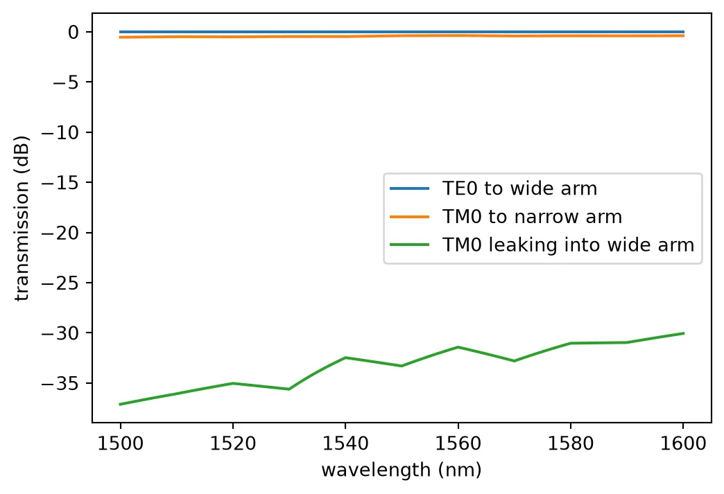

TM0 conversion loss 0.36 to 0.54 dB over 1500-1600 nm

The commented cell below runs the TM path by FDTD and writes the data file: TM0 launched at the input, 10 cells per wavelength, with 20 nm cells across the 200 nm gap over the whole coupler. The group delay uses an average group index of 4.2 over the 460 um device.

# # TM path by FDTD: TM0 in at P0, the two TE0 outputs measured
# xb, xc = psr_dims["la"] + psr_dims["lb"], psr_dims["la"] + psr_dims["lb"] + psr_dims["lc"]
# y_gap = -(psr_dims["rib_out"] + psr_dims["broad_end"]) / 4 - psr_dims["gap"] / 2
# gap_mesh = td.MeshOverrideStructure(
#     geometry=td.Box(center=((xb + xc) / 2, y_gap, 0.11), size=(xc - xb, psr_dims["gap"] + 0.3, 0.3)),
#     dl=(None, 0.02, None),
# )
# psr_fdtd = psr(
#     model=pf.Tidy3DModel(
#         grid_spec=td.GridSpec.auto(wavelength=lda0, min_steps_per_wvl=10, override_structures=[gap_mesh]),
#         verbose=False,
#     )
# )
# wl_fdtd = np.linspace(1.50, 1.60, 11)
# s = psr_fdtd.s_matrix(pf.C_0 / wl_fdtd, model_kwargs={"inputs": ["P0@1"]})
# length = sum(psr_dims[k] for k in ("la", "lb", "lc", "ld"))
# with open("misc/coherent_rx_psr.json", "w") as file:
#     json.dump(dict(wl=wl_fdtd.tolist(), tm_cro=np.abs(s[("P0@1", "P2@0")]).tolist(),
#                    tm_thr=np.abs(s[("P0@1", "P1@0")]).tolist(), tau_ps=4.2 * length / pf.C_0 * 1e12), file)

TM0 reaches the narrow arm with 0.4 to 0.5 dB of loss and leaks between $-37$ and $-30$ dB into the wide arm, so after the PSR the two polarizations are separated by 30 dB or more.

90 degree hybrid

The hybrid mixes the signal $E_s$ of one polarization with the LO $E_\text{LO}$ and produces four outputs, $E_s \pm E_\text{LO}$ and $E_s \pm j E_\text{LO}$ up to a common factor. Two balanced photodiode pairs on these outputs give the in-phase and quadrature beat, the real and imaginary parts of $E_s E_\text{LO}^*$. The design is that of Guan et al. [3], as built in the 90 degree optical hybrid example, which also compares the circuit of sub-components used here with an FDTD simulation of the whole hybrid.

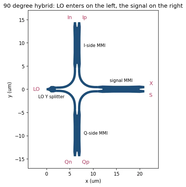
It works with one property of a 2x2 MMI: light entering one input leaves both outputs with equal power, and the output on the far side, the cross port, lags the near one, the bar port, by 90 degrees. The hybrid uses three of them and a Y splitter:

1. The Y splitter divides the LO into two equal halves, in phase.
2. The signal enters the right-hand MMI, which splits it into two halves 90 degrees apart.
3. Each signal half meets one LO half in a second MMI, the upper one on the I side and the lower one on the Q side. Each of these MMIs combines its two inputs into a bar and a cross output, $(E_s + j E_\text{LO})/\sqrt{2}$ and $(j E_s + E_\text{LO})/\sqrt{2}$ up to a common factor, whose powers differ by the in-phase beat $\mathrm{Re}(E_s E_\text{LO}^*)$ with opposite signs.
4. The signal reaching the Q-side MMI carries the extra 90 degrees of step 2, so its beat is the quadrature one, $\mathrm{Im}(E_s E_\text{LO}^*)$.

The drawing shows the hybrid with its ports and the role of each MMI. The LO enters on the left and the signal on the right; X is the unused second input of the signal MMI.

The figures of merit are:

• Phase error, the deviation of the I-to-Q phase from 90 degrees;
• Imbalance, the power ratio of the two outputs of a pair;
• Common-mode rejection ratio (CMRR), the fraction of the common power that survives the subtraction in a balanced pair, which lets LO intensity noise into the signal.

Each sub-component gets an FDTD model on the technology of this series, and the hybrid is a circuit of them. The access waveguides of the MMI sit close together, so the strip port window is narrowed to 0.9 um, which keeps the neighbouring guide out of the port mode.

wavelengths = np.linspace(1.530, 1.565, 36)  # C band, the hybrid's operating band
freqs = pf.C_0 / wavelengths
strip = tech_rx.ports["Strip_TE"].copy()
strip.width = 0.9  # Narrow window: the MMI access waveguides are close together
core_width = 0.5

# 2x2 MMI of Guan et al.: a 1.48 um wide body with tapered access waveguides
w = (1.48, 1.48, 1.6, 0.5, 0.7, 0.2)
l = (1, 2.4, 1.6)
v = np.array(
    (
        (-l[1] - l[2], w[5] / 2),
        (-l[0] - l[1] - l[2], (w[5] + w[4] - w[3]) / 2),
        (-l[0] - l[1] - l[2], (w[5] + w[4] + w[3]) / 2),
        (-l[1] - l[2], w[5] / 2 + w[4]),
        (-l[2], w[0] / 2),
        (0, w[1] / 2),
        (0, 0),
        (-l[1] - l[2], 0),
    )
)
# One quadrant of the outline, mirrored into the other three
mmi_core = pf.boolean(
    [
        pf.Polygon(v),
        pf.Polygon(-v),
        pf.Polygon(v * np.array((-1, 1))),
        pf.Polygon(v * np.array((1, -1))),
    ],
    [],
    "+",
)[0]
mmi2x2 = pf.Component("MMI")
mmi2x2.add("Si", mmi_core)
mmi2x2.add_port(mmi2x2.detect_ports([strip]))
# The four-fold symmetry of the MMI means one input is enough
mmi_symmetries = [
    ("P1", "P0", "P3", "P2"),
    ("P2", "P3", "P0", "P1"),
    ("P3", "P2", "P1", "P0"),
]
mmi2x2.add_model(
    pf.Tidy3DModel(port_symmetries=mmi_symmetries, verbose=False), "Tidy3D"
)

# Y splitter for the LO, 2 um long
w_y = np.array((0.5, 0.5, 0.6, 0.7, 0.9, 1.26, 1.4, 1.4, 1.4, 1.4, 1.31, 1.2, 1.2))
y_length = 2.0
y_out = (w_y[-1] - core_width) / 2
v_y = np.vstack((np.linspace(0, y_length, len(w_y)), -0.5 * w_y)).T
y_splitter = pf.Component("Y_SPLITTER")
y_splitter.add("Si", pf.Polygon(np.vstack((v_y, v_y[::-1] * np.array((1, -1))))))
# Two short stubs, so the output port planes see single waveguides
y_splitter.add(
    "Si",
    pf.Path((y_length, y_out), w_y[0]).segment((0.1, 0), relative=True),
    pf.Path((y_length, -y_out), w_y[0]).segment((0.1, 0), relative=True),
)
found = sorted(
    y_splitter.detect_ports([strip], on_boundary="x"),
    key=lambda p: (p.center[0], p.center[1]),
)
for name, port in zip(("P0", "P1", "P2"), found):
    y_splitter.add_port(port, name)
y_splitter.add_model(
    pf.Tidy3DModel(port_symmetries=[("P0", "P2", "P1")], verbose=False), "Tidy3D"
)

# Euler bends that route the LO and signal between the MMIs
bend = pf.parametric.bend(
    port_spec=strip,
    radius=4.0,
    angle=90,
    euler_fraction=0.5,
    name="BEND",
    model=pf.Tidy3DModel(port_symmetries=[("P1", "P0")], verbose=False),
)

# Straight fillers that match the Y-splitter output pitch to the MMI input pitch
m_gap = mmi2x2.ports["P1"].center[1] - mmi2x2.ports["P0"].center[1]
y_gap = y_splitter.ports["P2"].center[1] - y_splitter.ports["P1"].center[1]
fill = pf.parametric.straight(
    port_spec=strip,
    length=0.5 * (m_gap - y_gap),
    name="FILLER",
    model=pf.WaveguideModel(verbose=False),
)

hybrid = pf.component_from_netlist(
    {
        "name": "HYBRID",
        "instances": {
            "y": y_splitter,
            "mmi-top": mmi2x2,
            "mmi-bottom": mmi2x2,
            "mmi-right": mmi2x2,
            "b0": bend,
            "b1": bend,
            "b2": bend,
            "b3": bend,
            "fill0": fill,
            "fill1": fill,
        },
        "connections": [
            (("b0", "P1"), ("y", "P1")),
            (("b1", "P0"), ("y", "P2")),
            (("fill0", "P0"), ("b0", "P0")),
            (("fill1", "P0"), ("b1", "P1")),
            (("mmi-bottom", "P0"), ("fill0", "P1")),
            (("mmi-top", "P1"), ("fill1", "P1")),
            (("b2", "P1"), ("mmi-bottom", "P1")),
            (("b3", "P0"), ("mmi-top", "P0")),
            (("mmi-right", "P0"), ("b2", "P0")),
        ],
        "ports": [
            ("y", "P0", "LO"),
            ("mmi-bottom", "P2", "Qn"),
            ("mmi-bottom", "P3", "Qp"),
            ("mmi-top", "P2", "Ip"),
            ("mmi-top", "P3", "In"),
            ("mmi-right", "P2", "S"),
            ("mmi-right", "P3", "X"),
        ],
        "models": [(pf.CircuitModel(verbose=False), "Circuit")],
    }
)
viewer(hybrid)

LayoutSchematic

s_hy = hybrid.s_matrix(freqs)

# The FDTD results become the models of the hybrid and of its Y splitter, which also splits the LO
# on the die. Each model keeps the paths from an input to an output, in both directions.
s_y = y_splitter.s_matrix(freqs)
for cell, s, inputs in ((y_splitter, s_y, ("P0",)), (hybrid, s_hy, ("LO", "S", "X"))):
    is_input = lambda key: key.split("@")[0] in inputs
    through = {k: v for k, v in s.elements.items() if is_input(k[0]) != is_input(k[1])}
    model = pf.DataModel(pf.SMatrix(freqs, through), interpolation_method="linear")
    # Use a constant matrix as time stepper: both delay light by less than one time step of the link
    model.time_stepper = pf.SMatrixTimeStepper(
        min_poles=0, max_poles=0, feedthrough=True, delays=0.0, passive=False
    )
    cell.add_model(model, "FDTD data")

# Figures of merit for an input on the LO and on the signal port
fom = {}
for port_in in ("LO", "S"):
    p = {
        k: np.abs(s_hy[(f"{port_in}@0", f"{k}@0")]) ** 2
        for k in ("Ip", "In", "Qp", "Qn")
    }
    fom[f"insertion loss, {port_in} (dB)"] = -10 * np.log10(sum(p.values()))
    for b in ("I", "Q"):
        fom[f"imbalance {b}, {port_in} (dB)"] = 10 * np.log10(p[b + "p"] / p[b + "n"])
        cmrr = np.abs(p[b + "p"] - p[b + "n"]) / (p[b + "p"] + p[b + "n"])
        fom[f"CMRR {b}, {port_in} (dB)"] = 20 * np.log10(cmrr)

# Phase error: the I-to-Q phase of the beat, minus 90 degrees
phi = lambda a, b: np.angle(s_hy[(f"{a}@0", f"{b}@0")], deg=True)
phase_error = (
    90 - phi("S", "Qp") + phi("LO", "Qn") - phi("LO", "In") + phi("S", "Ip") + 180
) % 360 - 180
fom["phase error (deg)"] = phase_error

print(f"{'over 1530-1565 nm':32s}  min      max")
for key, value in fom.items():
    print(f"{key:32s} {np.min(value):6.2f}  {np.max(value):6.2f}")

fig, ax = plt.subplots(1, 2, figsize=(11, 3.6))
ax[0].plot(wavelengths * 1e3, phase_error)
ax[0].set_ylabel("phase error (deg)")
for port_in in ("LO", "S"):
    ax[1].plot(
        wavelengths * 1e3,
        fom[f"CMRR I, {port_in} (dB)"],
        label=f"I pair, {port_in} input",
    )
ax[1].set_ylabel("CMRR (dB)")
ax[1].legend()
for a in ax:
    a.set_xlabel("wavelength (nm)")
plt.show()

over 1530-1565 nm                 min      max
insertion loss, LO (dB)            0.22    0.31
imbalance I, LO (dB)               0.49    0.50
CMRR I, LO (dB)                  -25.00  -24.89
imbalance Q, LO (dB)               0.49    0.50
CMRR Q, LO (dB)                  -25.00  -24.89
insertion loss, S (dB)             0.23    0.39
imbalance I, S (dB)               -0.51   -0.48
CMRR I, S (dB)                   -25.11  -24.72
imbalance Q, S (dB)               -0.50   -0.48
CMRR Q, S (dB)                   -25.14  -24.82
phase error (deg)                  0.25    1.18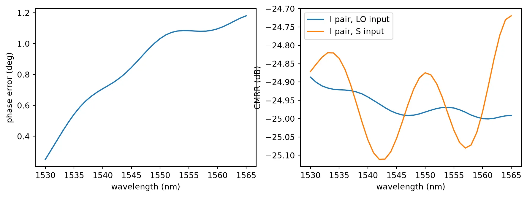

The phase error stays below 1.2 degrees over the C band, and the insertion loss is 0.2 to 0.4 dB. Each balanced pair is unbalanced by about half a decibel, the same for the LO and the signal, which puts the CMRR near $-25$ dB. The receiver DSP orthogonalizes I and Q and removes the small phase error, and a CMRR below $-20$ dB keeps LO intensity noise far below the signal. The complex S matrix of the hybrid is now its model, so these figures go into the link page as they are. The time stepper of the model is a constant matrix, as for the MMI of the transmitter page: the hybrid delays light by less than one time step of the link, and its response is flat over the signal band.

Photodiode and amplifier

The photodiode is the lateral p-i-n germanium detector of Chen et al. [4]: a 500 nm wide, 160 nm thick germanium strip 14.2 um long, on a silicon pad that carries the junction. The p and n implants meet under the centre of the germanium, and the contacts are on the silicon outside it, so no metal touches the germanium and no implant is placed in it. A silicon taper with a polysilicon strip on top brings the light up from the 500 nm input strip into the germanium. The paper reports 0.74 A/W at 1550 nm, a bandwidth beyond 67 GHz at $-1$ V and 3.6 nA of dark current, which the model below uses.

The cell below draws the photodiode as a parametric component. Besides its optical input P0, the cell has an electrical output E0 and the model of the front end: the photodiode with its TIA, the 80 GHz amplifier of Gläsel et al. [5] that the next sections describe. The arguments set the two bandwidths and the seed of the noise. Each photodiode of the chip gets its own seed, so the eight photodiodes draw independent noise.

ge_length = 14.2  # Germanium length (um)
ge_width = 0.5  # Germanium width (um)
si_half_width = 2.2  # Silicon pad under and beside the germanium, each side (um)
contact_offset = 1.2  # Inner edge of the contact implants (um)
taper_length = 10.0  # Input taper length (um)
wg_width = 0.5  # Input wire width (um), the strip of the technology

responsivity = 0.74  # A/W at 1550 nm, -1 to -2 V
dark_current = 3.6e-9  # Photodiode dark current (A)
saturation_current = 1e-3  # Photocurrent where the response starts to compress (A)
tia_gain = 10 ** (74 / 20)  # 74 dB-ohm transimpedance (V/A)
tia_noise = 12.2e-12  # TIA input noise density (A/rtHz)

@pf.parametric_component(name_prefix="PD_CHEN")
def ge_photodiode(*, f_pd=67e9, f_tia=80e9, seed=0):
    pd = pf.Component()
    h = si_half_width
    # Silicon: input wire, taper to the full pad, then the pad under the germanium
    pd.add(
        "Si",
        pf.Polygon(
            [
                (-taper_length, -wg_width / 2),
                (0, -h),
                (ge_length, -h),
                (ge_length, h),
                (0, h),
                (-taper_length, wg_width / 2),
            ]
        ),
    )
    # Polysilicon taper on top of the silicon taper, ending at the germanium width
    pd.add(
        "Poly Si",
        pf.Polygon(
            [
                (-taper_length, -0.1),
                (0, -ge_width / 2),
                (0, ge_width / 2),
                (-taper_length, 0.1),
            ]
        ),
    )
    pd.add("Ge", pf.Rectangle((0, -ge_width / 2), (ge_length, ge_width / 2)))
    # Lateral junction: n on one side, p on the other, meeting under the germanium centre
    pd.add(
        "Si n",
        pf.Rectangle((0, -h), (ge_length, 0)),
        "Si p",
        pf.Rectangle((0, 0), (ge_length, h)),
    )
    pd.add(
        "Si n++",
        pf.Rectangle((0, -h), (ge_length, -contact_offset)),
        "Si p++",
        pf.Rectangle((0, contact_offset), (ge_length, h)),
    )
    # Tungsten plugs on the contact implants and M1 above them
    for sign in (-1, 1):
        y0, y1 = sorted((sign * (contact_offset + 0.2), sign * (h - 0.2)))
        pd.add(
            "Contact",
            pf.Rectangle((0.5, y0), (ge_length - 0.5, y1)),
            "M1",
            pf.Rectangle((0.0, y0 - 0.2), (ge_length, y1 + 0.2)),
        )
    pd.add_terminal(
        pf.Terminal("M1", pf.Rectangle((0.0, -h), (ge_length, -contact_offset))),
        "CATHODE",
    )
    pd.add_terminal(
        pf.Terminal("M1", pf.Rectangle((0.0, contact_offset), (ge_length, h))), "ANODE"
    )
    # Optical input on the strip, and the electrical output of the front end on the anode
    pd.add_port(pf.Port((-taper_length, 0), 0, "Strip_TE"), "P0")
    pd.add_port(
        pf.Port(
            pd.terminals["ANODE"].center(),
            90,
            pf.virtual_port_spec(classification="electrical"),
        ),
        "E0",
    )

    # Front end: the two poles in cascade are one second-order filter
    f_filter = np.sqrt(f_pd * f_tia)
    front_end = pfa.photodiode(
        responsivity=responsivity,
        gain=tia_gain,
        dark_current=dark_current,
        thermal_noise=tia_noise**2,  # A^2/Hz
        saturation_current=saturation_current,
        filter_frequency=f_filter,  # Natural frequency of the filter (Hz)
        filter_quality=f_filter / (f_pd + f_tia),  # Quality factor of the filter
        seed=seed,
    )
    # Take the optical and the electrical model of the abstract photodiode
    pd.add_model(front_end.models["Termination"], "Front end")
    pd.add_model(
        front_end.models["Termination (electrical)"],
        "Termination (electrical)",
        set_active="electrical",
    )
    return pd

pd_cell = ge_photodiode()
viewer(pd_cell)

Junction capacitance

The bandwidth of a photodiode is limited by the carrier transit across the depletion region and by the RC time of its capacitance with the load. The charge solver gives the capacitance from the drawn cell: Component.extrude with classification="electrical" returns the solids of the photodiode with the electrical half of each material of the technology page, so the implants carry their doping and the plugs are conductors without any further definition. The undoped germanium is fully depleted at reverse bias, so the technology gives it a dielectric of permittivity 16 in the charge solve. The capacitance is computed per unit length at bias steps from 0 to $-2$ V.

bias = [0.0, 0.5, 1.0, 1.5, 2.0]  # Reverse bias (V)
x_cut = ge_length / 2  # Cross-section halfway along the germanium

# Every solid of the drawn photodiode, with the electrical half of each material from the technology:
# doped silicon from the implants, germanium, oxide and tungsten. The two plugs are named, because a
# voltage condition attaches to a named structure; the cathode is on the n side, at negative y.
charge_structures = [
    (
        s.updated_copy(name="cathode" if s.geometry.bounds[0][1] < 0 else "anode")
        if s.medium.name == "W"
        else s
    )
    for s in (
        solid.to_tidy3d() for solid in pd_cell.extrude(classification="electrical")
    )
]

# The simulation is a plane across the germanium: nothing varies along the photodiode. It spans the
# silicon pad and stops below M1, so only the plugs reach the contacts.
charge_sim = td.HeatChargeSimulation(
    center=(x_cut, 0, 0.3),
    size=(0, 2 * si_half_width + 0.6, 1.8),
    structures=charge_structures,
    medium=sio2["electrical"],
    monitors=[
        # Capacitance per unit length, from the charge stored at each bias
        td.SteadyCapacitanceMonitor(
            center=(x_cut, 0, 0.3), size=(0, td.inf, td.inf), name="cap"
        )
    ],
    boundary_spec=[
        # Ground the anode and raise the cathode, which reverse-biases the junction
        td.HeatChargeBoundarySpec(
            condition=td.VoltageBC(source=td.DCVoltageSource(voltage=0)),
            placement=td.StructureBoundary(structure="anode"),
        ),
        td.HeatChargeBoundarySpec(
            condition=td.VoltageBC(source=td.DCVoltageSource(voltage=bias)),
            placement=td.StructureBoundary(structure="cathode"),
        ),
    ],
    grid_spec=td.DistanceUnstructuredGrid(
        dl_interface=0.004,  # Element size at interfaces (um)
        dl_bulk=0.05,  # Far from interfaces nothing changes quickly
        distance_interface=0.01,
        distance_bulk=0.3,
        relative_min_dl=0,
        sampling=500,
        mesh_refinements=[
            # 3 nm elements over the junction under the germanium, where the depletion edge sits
            td.GridRefinementRegion(
                center=(x_cut, 0, 0.19),
                size=(0, 0.8, 0.38),
                dl_internal=0.003,
                transition_thickness=0.05,
            )
        ],
    ),
    # Steady-state drift-diffusion at room temperature, with Fermi-Dirac statistics for the 1e20 implants
    analysis_spec=td.IsothermalSteadyChargeDCAnalysis(
        temperature=300, fermi_dirac=True
    ),
)
charge_data = web.run(charge_sim, task_name="pd_capacitance", verbose=False)

# Capacitance per length from the electron and hole charge, in fF/um
cap = charge_data["cap"]
c_per_um = 0.5 * (
    np.abs(cap.electron_capacitance.data) + np.abs(cap.hole_capacitance.data)
)
c_device = c_per_um * ge_length
for v_b, c_b in zip(cap.electron_capacitance.coords["v"].data, c_device):
    print(f"reverse bias {v_b:.1f} V: {c_b:.2f} fF")

# RC limit with a 50 ohm load, at -2 V
f_rc = 1 / (2 * np.pi * 50 * c_device[-1] * 1e-15)
print(f"RC limit with 50 ohm at -2 V: {f_rc * 1e-9:.0f} GHz")

reverse bias 0.0 V: 7.59 fF
reverse bias 0.5 V: 7.07 fF
reverse bias 1.0 V: 6.22 fF
reverse bias 1.5 V: 5.66 fF
reverse bias 2.0 V: 5.43 fF
RC limit with 50 ohm at -2 V: 586 GHz

The capacitance is a few femtofarads, so the RC limit is several hundred gigahertz and the bandwidth is set by the carrier transit across the 0.5 um germanium, which is why the paper measures beyond 67 GHz. The charge solve gives 5.4 fF at $-2$ V against 6.2 fF reported by Chen et al., whose device also has the capacitance of its pads and its contact wiring.

The receiver front end

Each photodiode feeds a TIA. The amplifier here is a SiGe linear TIA with 74 dB-ohm of transimpedance and an input noise density of 12.2 pA/$\sqrt{\text{Hz}}$, values typical of linear TIAs for coherent receivers, and an 80 GHz bandwidth, as in the 128 GBd receiver of Gläsel et al. [5]. The photodiode pole at 67 GHz and the amplifier pole at 80 GHz in cascade are one second-order low-pass filter with

$$f_0 = \sqrt{f_\text{PD} f_\text{TIA}}, \qquad Q = \frac{f_0}{f_\text{PD} + f_\text{TIA}},$$

and photodiode from the abstract library takes exactly these: a responsivity, a gain in volts per ampere, the dark current, the thermal-noise density of the amplifier, a saturation current and a second-order filter. The photodiode cell above already carries this model. The cell below measures its response with small-signal tones in the time domain.

# The photodiode cell with a fixed noise sequence, so the measured response repeats
front_end = ge_photodiode(seed=1)

# Small-signal tones: 0.2 mW average (0.15 mA, well below saturation) with 10 % modulation
dt = 1 / 2e12
t = np.arange(40000) * dt
p_avg, depth = 2e-4, 0.1
stepper = front_end.models["Front end"].time_stepper
stepper.setup(front_end, dt, carrier_frequency=f0, show_progress=False)
tones = np.array([1, 10, 20, 30, 40, 45, 50, 55, 60, 70, 80, 100]) * 1e9
response = []
for f in tones:
    stepper.reset()
    power = p_avg * (1 + depth * np.sin(2 * np.pi * f * t))
    out = stepper.step(
        pf.TimeSeries(values={"P0@0": np.sqrt(power)}, time_step=dt),
        show_progress=False,
    )
    # Wave amplitude to volts on 50 ohm
    v = np.real(np.asarray(out["E0@0"])) * np.sqrt(50)
    keep = t > 0.2 * t[-1]  # Skip the filter's start transient
    a = np.c_[
        np.sin(2 * np.pi * f * t[keep]),
        np.cos(2 * np.pi * f * t[keep]),
        np.ones(keep.sum()),
    ]
    coef = np.linalg.lstsq(a, v[keep], rcond=None)[0]
    response.append(np.hypot(coef[0], coef[1]) / (responsivity * p_avg * depth))
response = np.array(response)
response_db = 20 * np.log10(response / response[0])
f3db = np.interp(-3, response_db[::-1], tones[::-1])
print(f"transimpedance {20 * np.log10(response[0]):.1f} dB-ohm at 1 GHz")
print(f"front-end 3 dB bandwidth {f3db * 1e-9:.1f} GHz")

fig, ax = plt.subplots(1, 1, figsize=(6, 4))
ax.plot(tones * 1e-9, response_db, "o-")
ax.axhline(-3, color="0.5", ls="--", lw=1)
ax.set_xlabel("frequency (GHz)")
ax.set_ylabel("response (dB)")
ax.set_title("photodiode and TIA")
plt.show()

transimpedance 73.5 dB-ohm at 1 GHz
front-end 3 dB bandwidth 48.7 GHz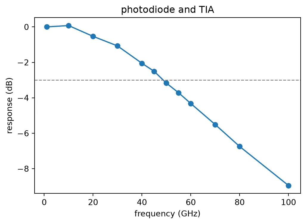

The front end has a 3 dB bandwidth of about 47 GHz: the two poles in cascade give 46.9 GHz, and the tone measurement reads it to within the noise of the TIA. This is below half the symbol rate, so the receiver relies on the equalizer of the DSP, as commercial coherent receivers at this rate do. The link page measures what the 47 GHz costs in OSNR by comparing it with an 80 GHz front end.

What comes next

The receiver library is complete. The layout page draws the transmitter and receiver chips from the two libraries and checks them, and the link page simulates the link.