Differential Coplanar Waveguide
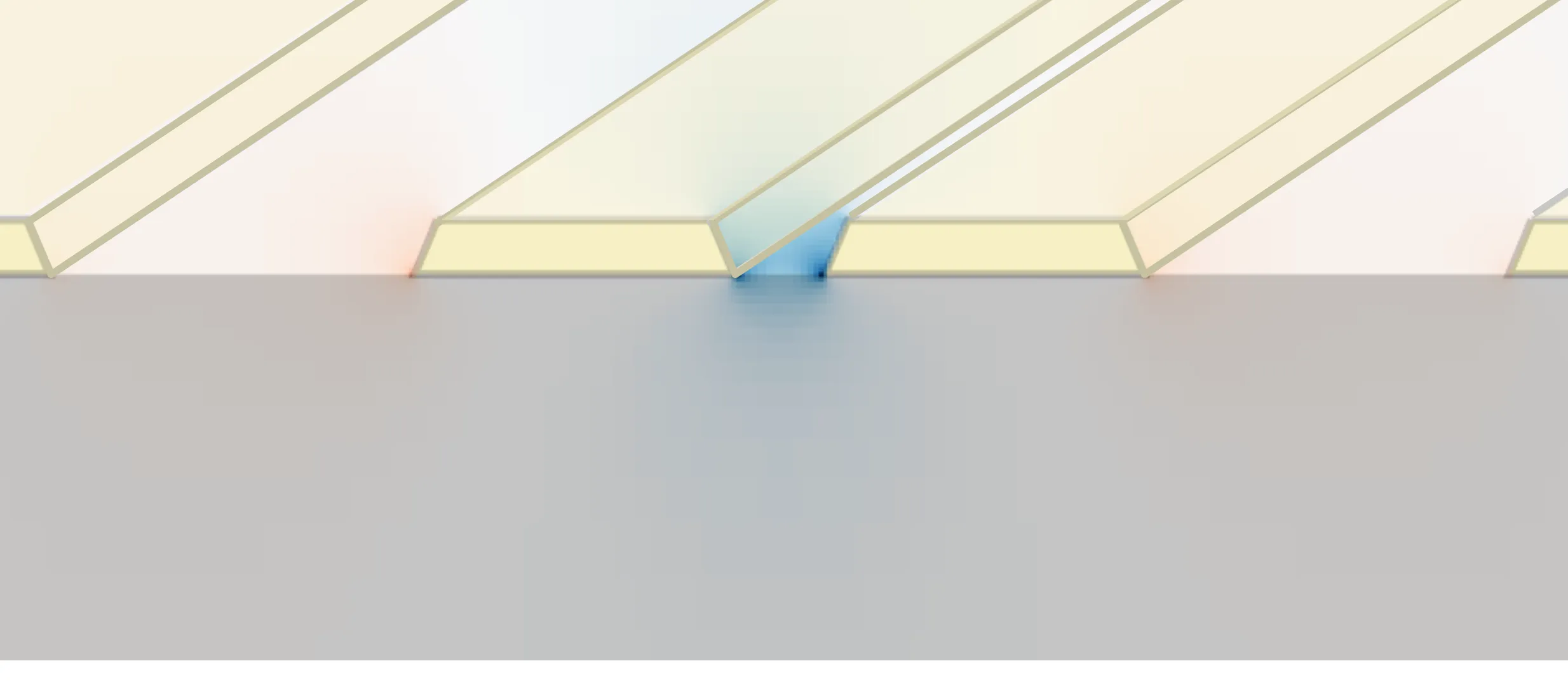
In this notebook, we simulate and analyze a differential coplanar waveguide (CPW) structure using both mode solving and time-domain FDTD methods within PhotonForge.
Our goal is to extract key transmission line properties—impedance, effective index, and loss—for a differential pair over a wide frequency range. We benchmark the results against a reference simulation from another commercial software to validate accuracy.
We start by defining the physical dimensions and material parameters of the CPW layout. All values are selected to match a reference example. The impedance results are compared across varying signal-to-signal spacings to demonstrate consistency with expected differential behavior.
Later in the notebook, we simulate a 1 cm differential CPW line using both FDTD and a Waveguide-based model, and compare their scattering parameters to verify agreement.
import numpy as npimport photonforge as pfimport tidy3d as tdfrom matplotlib import pyplot as pltfrom tidy3d.plugins.dispersion import FastDispersionFitter
td.config.logging.level = "ERROR"pf.config.default_mesh_refinement = 30  # Set default mesh refinement
Parameters for Differential CPW Geometry
Section titled “Parameters for Differential CPW Geometry”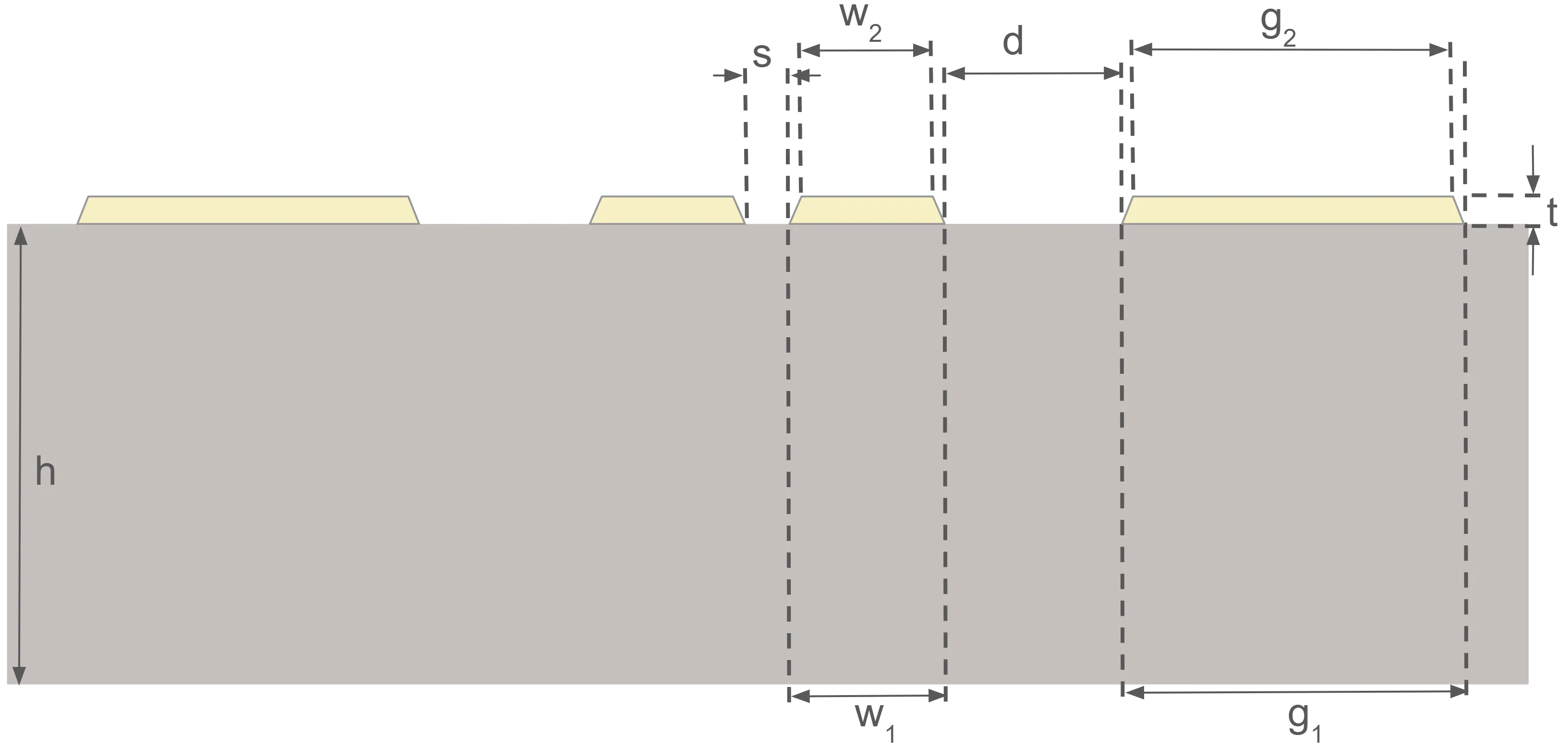
In this section, we define the physical and electrical parameters of the differential coplanar waveguide (CPW) structure based on the diagram provided above. We set the conductor and substrate properties, geometry dimensions, and simulation frequency range. The units are converted using the mil factor (1 mil = 25.4 microns), which is commonly used in PCB and microwave engineering.
f_min = 1e9  # minimum frequency (Hz)f_max = 50e9  # maximum frequency (Hz)mil = 25.4  # conversion factor: 1 mil = 25.4 microns
losstan_sub = 0.015  # substrate loss tangentcond_metal = 41  # metal conductivityeps_sub = 4.2  # relative permittivity of substrate
h = 8.5 * mil  # substrate thicknessw1 = 7 * mil  # signal width (bottom)w2 = 6 * mil  # signal width (top)s = 2 * mil  # spacing between signal linesg1 = 101 * mil  # ground width (bottom)g2 = 100 * mil  # ground width (top)d = 8 * mil  # gap between signal and groundt = 1.2 * mil  # conductor thickness
freqs = np.linspace(f_min, f_max, 21)  # frequency sweep points
Simple PCB Technology
Section titled “Simple PCB Technology”We define a reusable Technology class that represents a simple PCB stack for our differential CPW. This includes the substrate and transmission line (TL) metal layers. The function allows us to customize key physical properties such as conductor thickness, substrate thickness, and sidewall angle. The stack-up also specifies materials used for the substrate, metal, and surrounding dielectric opening. This technology will be passed to layout and simulation components later.
_Medium = td.components.medium.MediumType  # type alias for medium input
def basic_pcb_tech(    *,    sidewall_angle: float = 22.6,  # sidewall taper angle (deg)    sub_thickness: float = 8.5 * mil,  # substrate thickness (microns)    tl_thickness: float = 1.2 * mil,  # conductor thickness (microns)    substrate: _Medium = td.Medium(        permittivity=4.2, name="Substrate"    ),  # substrate material    tl_metal: _Medium = td.PECMedium(),  # metal for transmission lines    opening: _Medium = td.Medium(        permittivity=1.0, name="Opening"    ),  # surrounding dielectric) -> pf.Technology:    # Layers    layers = {        "TL": pf.LayerSpec(            layer=(21, 0),  # GDS layer for metal            description="Metal transmission lines",            color="#eadb0718",            pattern="\\",        ),    }
    # Extrusion specifications    bounds = pf.MaskSpec()  # empty mask for entire domain    tl_mask = pf.MaskSpec((21, 0))  # mask for transmission lines    extrusion_specs = [        pf.ExtrusionSpec(bounds, substrate, (-sub_thickness, 0)),  # extrude substrate        pf.ExtrusionSpec(            tl_mask, tl_metal, (0, tl_thickness), sidewall_angle        ),  # extrude TLs    ]
    # Create and return PCB technology stack    technology = pf.Technology("PCB", "0", layers, extrusion_specs, {}, opening)
    return technology
We compute the effective sidewall angle based on the difference between ground and signal widths, assuming symmetric metal tapering. This angle is then used to instantiate our PCB technology stack. Finally, we set this technology as the default in PhotonForge for use in subsequent component definitions and simulations.
# compute metal sidewall angle in degreessidewall_angle = np.degrees(np.arctan((w1 - w2) / 2 / t))
# instantiate PCB techtech = basic_pcb_tech(sidewall_angle=sidewall_angle, sub_thickness=h)pf.config.default_technology = tech  # set as default technology
Port Definition
Section titled “Port Definition”We define a PortSpec object for the differential CPW using the smallest signal spacing value. This specification includes metal trace profiles as well as paths used to compute voltage and current integrals for impedance extraction.
To better understand the setup, we visualize the port cross-section at the simulation center and overlay the voltage and current integration paths. This helps confirm that the field sampling and excitation definitions are aligned with the geometry and symmetry of the structure.
dcpw_spec = pf.PortSpec(    description="Differential CPW transmission line",    width=2 * g1 + s + 2 * w1 + 2 * d - 1 * mil,  # simulation domain width    limits=(-100 * mil, 100 * mil),  # z-axis extent    num_modes=1,  # number of target modes    added_solver_modes=0,  # extra solver modes    polarization="",  # default polarization    target_neff=2,  # expected effective index    path_profiles={  # cross-sectional layout        "gnd0": (g2, w1 + d + (s + g1) / 2, (21, 0)),        "gnd1": (g2, -(w1 + d + (s + g1) / 2), (21, 0)),        "signal0": (w2, -(s + w1) / 2, (21, 0)),        "signal1": (w2, (s + w1) / 2, (21, 0)),    },    voltage_path=[  # voltage integration line        (-s / 2 - (w1 - w2) / 2, t / 2),        (s / 2 + (w1 - w2) / 2, t / 2),    ],    current_path=[  # current integration loop        (w1 + s / 2 + d / 2, 2 * t),        (0, 2 * t),        (0, -t),        (w1 + s / 2 + d / 2, -t),    ],)
ax = pf.tidy3d_plot(dcpw_spec, frequency=freqs[0])  # plot port geometryic = dcpw_spec.to_tidy3d_impedance_calculator()  # create impedance calculator
_ = ic.voltage_integral.plot(ax=ax, x=0)  # overlay voltage path_ = ic.current_integral.plot(ax=ax, x=0)  # overlay current loop
ax.set_xlim((-(s / 2 + w1 + 2 * d), (s / 2 + w1 + 2 * d)))  # limit x viewax.set_ylim((-25 * mil, 25 * mil))  # limit y viewplt.show()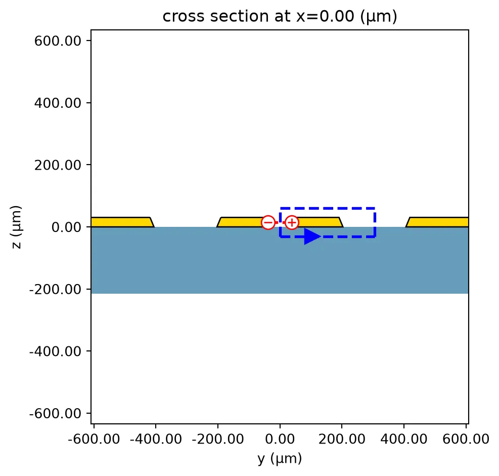
Inspect Ey Field to Verify Differential Mode
Section titled “Inspect Ey Field to Verify Differential Mode”To extract the correct differential impedance, we first visualize the electric field distribution for the computed mode. We verify the odd-symmetry voltage mode (i.e., the differential mode) by inspecting the Ey component of the fields.
We apply mirror symmetry to the simulation domain to ensure that the computed field profiles respect the physical symmetry of the differential structure. This not only reduces simulation size but also significantly improves the accuracy of impedance extraction.
cpw_solver = dcpw_spec.to_tidy3d(freqs) # solve for port modescpw_solver_sym = cpw_solver.updated_copy( simulation=cpw_solver.simulation.updated_copy( symmetry=(0, -1, 0), # apply y-symmetry ))mode_data = pf.port_modes(cpw_solver_sym) # extract mode field dataax = mode_data.plot_field("Ey", "real", f=freqs[0], robust=False)ax.set_xlim((-(s / 2 + w1 + 2 * d), (s / 2 + w1 + 2 * d))) # x-rangeax.set_ylim((-25 * mil, 25 * mil)) # y-rangeplt.show()Uploading task 'Mode-ModeSolver…'Starting task 'Mode-ModeSolver': https://tidy3d.simulation.cloud/workbench?taskId=mo-ec2a6ab5-0bc9-4f64-a9cd-4a31c2d9b907Downloading data from 'Mode-ModeSolver'…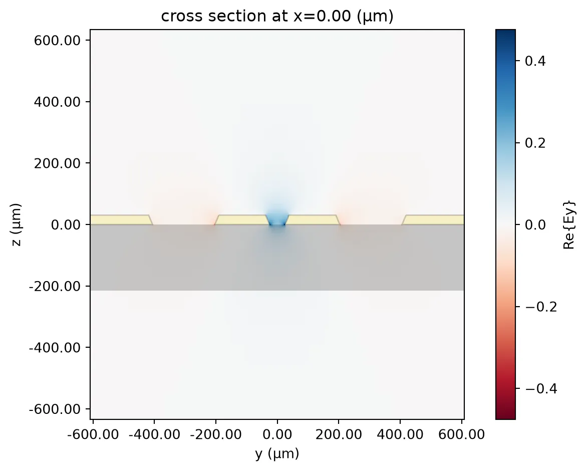
Extract Impedance and Effective Index
Section titled “Extract Impedance and Effective Index”After computing the differential mode, we extract its physical characteristics across the frequency range. These include:
- The real part of the differential impedance
Z₀, - The effective refractive index
n_eff, and
# differential impedancez0 = ic.compute_impedance(mode_data.data).real
n_eff = mode_data.data.n_eff  # effective index
fig, ax = plt.subplots(1, 2, figsize=(10, 4), tight_layout=True)
ax[0].plot(z0.f * 1e-9, z0)  # plot impedance vs frequencyax[0].set(xlabel="Frequencies (GHz)", ylabel="Re{Z₀} (Ω)")
ax[1].plot(freqs / 1e9, n_eff)  # plot effective indexax[1].set_xlabel("Frequency (GHz)")ax[1].set_ylabel("Effective index")
plt.show()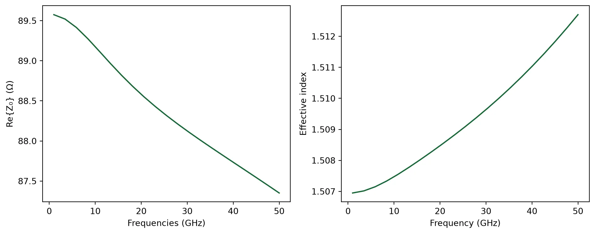
Benchmark Simulated Impedance Against Reference Data
Section titled “Benchmark Simulated Impedance Against Reference Data”In this section, we verify the simulated differential impedance of the CPW structure by comparing it with a reference simulation from another commercial software. We sweep the signal-to-ground spacing s and extract the real part of the differential impedance at the fundamental mode.
Here, we present an alternative approach for computing the impedance without enforcing symmetry directly in the simulation setup. In this case, small numerical asymmetries in the computed field profiles can cause slight differences in the calculated currents on the two signal traces. To account for this, we compute the impedance twice—once for each current path mirrored across the centerline—and then combine the results by summing their reciprocals. This method aligns with the definition of differential impedance, which is inversely proportional to the total current. The second call to pf.port_modes reuses the cached field solution and only recalculates the impedance, adding negligible overhead to the total simulation time.
It’s also important to note that the differential impedance Z₀(diff) is equal to twice the odd-mode impedance Z₀(odd) of a single-ended structure. As the spacing s increases, coupling between the signal lines decreases, and Z₀(diff) asymptotically approaches twice the single-ended value. In our case, the impedance saturates around 228 Ω, which aligns well with the expected 112 Ω of an isolated single-ended CPW line with the same geometry.
s_values = np.array([2, 6, 12, 20, 33, 50, 70, 100]) * mil  # sweep values for gap sz0_real_values = []  # store real parts of simulated impedance
for s in s_values:    spec = pf.PortSpec(        description="Differential CPW transmission line",        width=2 * g1 + s + 2 * w1 + 2 * d - 1 * mil,  # simulation domain width        limits=(-100 * mil, 100 * mil),  # z-axis extent        num_modes=1,  # number of target modes        added_solver_modes=0,  # extra solver modes        polarization="",  # default polarization        target_neff=2,  # expected effective index        path_profiles={  # cross-sectional layout            "gnd0": (g2, w1 + d + (s + g1) / 2, (21, 0)),            "gnd1": (g2, -(w1 + d + (s + g1) / 2), (21, 0)),            "signal0": (w2, -(s + w1) / 2, (21, 0)),            "signal1": (w2, (s + w1) / 2, (21, 0)),        },        voltage_path=[  # differential voltage path            (-s / 2 - (w1 - w2) / 2, t / 2),            (s / 2 + (w1 - w2) / 2, t / 2),        ],        current_path=[  # differential current loop            (w1 + s / 2 + d / 2, 2 * t),            (0, 2 * t),            (0, -t),            (w1 + s / 2 + d / 2, -t),        ],    )
    _, z0_1 = pf.port_modes(spec, [freqs[0]], impedance=True)    spec.current_path = [(-x, y) for x, y in spec.current_path]    _, z0_2 = pf.port_modes(spec, [freqs[0]], impedance=True)    z0 = 2 / (1 / z0_1 + 1 / z0_2)    z0_real_values.append(z0.isel(f=0).real.item())
# Reference data from another commercial simulationdata_ref = [    [2, 89.5],    [6, 124.3],    [10, 144.1],    [14, 158.2],    [18, 168.9],    [22, 177.4],    [26, 184.4],    [30, 190.2],    [34, 195.1],    [38, 199.3],    [42, 203.0],    [46, 206.2],    [50, 209.0],    [54, 211.5],    [58, 213.7],    [62, 215.8],    [66, 217.6],    [70, 219.3],    [74, 220.8],    [78, 222.2],    [82, 223.4],    [86, 224.6],    [90, 225.7],    [94, 226.7],    [98, 227.6],    [102, 228.5],]s_ref = [row[0] for row in data_ref]  # reference s valuesz0_ref = [row[1] for row in data_ref]  # reference impedance values
# Plot bothplt.figure()plt.plot(    s_values / mil, z0_real_values, marker="o", label="Simulated")  # simulation resultsplt.plot(s_ref, z0_ref, linestyle="--", label="Reference")  # reference curveplt.xlabel("s (µm)")plt.ylabel("Impedance (Ω)")plt.title("Differential CPW Impedance vs s")plt.legend()plt.grid(True)plt.show()
# Reset s to default vaules = 2 * mil
Uploading task 'Mode-ModeSolver…'Starting task 'Mode-ModeSolver': https://tidy3d.simulation.cloud/workbench?taskId=mo-ef1cdcfd-48eb-46f0-b471-a23dfff4174aDownloading data from 'Mode-ModeSolver'…Uploading task 'Mode-ModeSolver…'Starting task 'Mode-ModeSolver': https://tidy3d.simulation.cloud/workbench?taskId=mo-164ca7ad-96be-472c-bbfc-1227f70b48ecDownloading data from 'Mode-ModeSolver'…Uploading task 'Mode-ModeSolver…'Starting task 'Mode-ModeSolver': https://tidy3d.simulation.cloud/workbench?taskId=mo-2e1ab33f-cd31-4e10-8b9a-e62f69bd7da3Downloading data from 'Mode-ModeSolver'…Uploading task 'Mode-ModeSolver…'Starting task 'Mode-ModeSolver': https://tidy3d.simulation.cloud/workbench?taskId=mo-e8813c98-8fb0-4430-b470-5c895ad60eceDownloading data from 'Mode-ModeSolver'…Uploading task 'Mode-ModeSolver…'Starting task 'Mode-ModeSolver': https://tidy3d.simulation.cloud/workbench?taskId=mo-e29b7487-18b5-4994-9cb3-410de1c1c82eDownloading data from 'Mode-ModeSolver'…Uploading task 'Mode-ModeSolver…'Starting task 'Mode-ModeSolver': https://tidy3d.simulation.cloud/workbench?taskId=mo-de851d09-d649-471b-9d85-93bc66483a1aDownloading data from 'Mode-ModeSolver'…Uploading task 'Mode-ModeSolver…'Starting task 'Mode-ModeSolver': https://tidy3d.simulation.cloud/workbench?taskId=mo-c6dea874-d870-4d7f-8a02-2d719c3a2677Downloading data from 'Mode-ModeSolver'…Uploading task 'Mode-ModeSolver…'Starting task 'Mode-ModeSolver': https://tidy3d.simulation.cloud/workbench?taskId=mo-8884e734-bfc0-4e1e-9981-e956a59e739fDownloading data from 'Mode-ModeSolver'…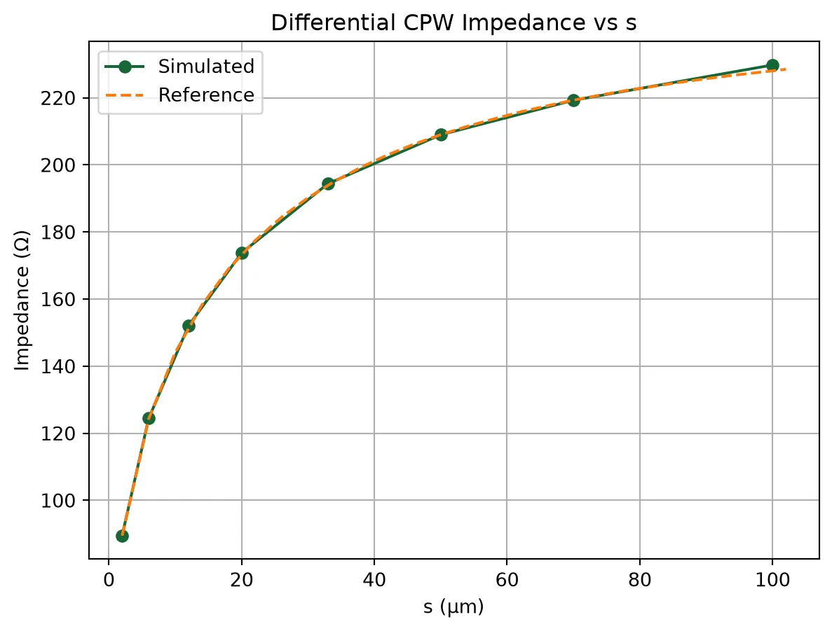
Lossy Differential CPW
Section titled “Lossy Differential CPW”In this section, we aim to simulate a lossy differential CPW transmission line by defining frequency-dependent models for both the conductor and the substrate. This allows us to capture realistic attenuation behavior due to dielectric and conductor losses.
We use a surface impedance fitting model for the metal, and a constant-loss-tangent dispersion model for the substrate. These models are valid over the frequency range of interest and will be used in both FDTD and mode solver simulations. Later, we will compare the results of these two approaches to assess consistency and accuracy.
lossy_metal: _Medium = td.LossyMetalMedium(    conductivity=cond_metal,  # metal conductivity    frequency_range=[f_min, f_max],  # fit range for frequency-dependent loss    fit_param=td.SurfaceImpedanceFitterParam(max_num_poles=16),  # fitting parameters)
lossy_substrate: _Medium = FastDispersionFitter.constant_loss_tangent_model(    eps_real=eps_sub,  # real permittivity of substrate    loss_tangent=losstan_sub,  # loss tangent for lossy dielectric    frequency_range=(f_min, f_max),  # frequency range of interest)
tech = basic_pcb_tech(    sidewall_angle=sidewall_angle,  # sidewall taper angle    sub_thickness=h,  # substrate thickness    substrate=lossy_substrate,  # frequency-dependent substrate model    tl_metal=lossy_metal,  # frequency-dependent metal model)pf.config.default_technology = tech  # set lossy tech as default
FDTD Simulation
Section titled “FDTD Simulation”We now simulate a 1 cm long differential CPW line using FDTD to evaluate its broadband S-parameter response. A field monitor is placed at the center of the line to record cross-sectional fields, which will later be used for mode inspection.
The structure is configured using the same port specification as the mode solver, and we apply mirror symmetry. After activating the model, we extract the full scattering matrix over the desired frequency range.
dcpw_length = 10000  # 1 cm line length in microns
field_monitor_yz = td.FieldMonitor(    center=(dcpw_length / 2, 0, 0),  # center of the transmission line    size=(0, td.inf, td.inf),  # yz cross-section    freqs=[20e9],  # monitor frequency    name="field_yz",  # monitor name)
dcpw_line = pf.parametric.straight(  # create straight DCPW line    port_spec=dcpw_spec,    length=dcpw_length,    name="DCPW Line",    model=pf.Tidy3DModel(        port_symmetries=[("E1", "E0")],        symmetry=(0, -1, 0),  # apply symmetry        monitors=[field_monitor_yz],  # add field monitor    ),)
dcpw_line.activate_model("Tidy3D")  # activate FDTD models_matrix = dcpw_line.s_matrix(frequencies=freqs)  # simulate and extract S-parameters
# pf.tidy3d_plot(dcpw_line, z=t / 2, hlim=(-500, 10100), vlim=(-2000, 2000))pf.tidy3d_plot(dcpw_line, plot_type="3d")
Uploading task 'E0@0…'Uploading task 'E0…'Uploading task 'E1…'Starting task 'E0@0': https://tidy3d.simulation.cloud/workbench?taskId=fdve-55fa2997-7c6a-4d84-aaed-a2d6fb217d48Starting task 'E1': https://tidy3d.simulation.cloud/workbench?taskId=mo-f1113993-36d5-4efe-ba61-9ca3a3720c4aStarting task 'E0': https://tidy3d.simulation.cloud/workbench?taskId=mo-5445bf1d-1126-4396-ace5-d9a2ab152a0bDownloading data from 'E0@0'…Downloading data from 'E0'…Downloading data from 'E1'…Simulate S-Matrix Using Waveguide Model
Section titled “Simulate S-Matrix Using Waveguide Model”We now switch from full-wave FDTD simulation to the Waveguide model, which reconstructs the transmission behavior using modal propagation constants such as effective index and loss. This model provides an efficient alternative for long uniform structures.
By activating the Waveguide model for our 1 cm differential CPW line, we compute the corresponding S-matrix across the frequency sweep. The result can be directly compared to the FDTD simulation for validation.
# Replace with a Waveguide modeldcpw_line.update(model=pf.WaveguideModel())
# simulate and extract S-parameterss_matrix_mode = dcpw_line.s_matrix(frequencies=freqs)
Uploading task 'Mode-DifferentialCPWtransmissionline…'Starting task 'Mode-DifferentialCPWtransmissionline': https://tidy3d.simulation.cloud/workbench?taskId=mo-3d8b63a5-e471-4cb3-84cd-6d6245867974Downloading data from 'Mode-DifferentialCPWtransmissionline'…Compare 3D FDTD RF Model and Waveguide Model
Section titled “Compare 3D FDTD RF Model and Waveguide Model”We finalize the comparison by plotting the transmission response of the differential CPW line obtained from both our GPU-accelerated RF FDTD solver and the Waveguide model (RF mode solver).
We plot the magnitude and phase of S21 for both approaches. Good agreement confirms the validity of using the Waveguide model as an efficient surrogate for full-wave simulations when the geometry is uniform and dispersion is captured accurately.
# Extract S-parameterss21 = s_matrix["E0@0", "E1@0"]  # FDTD results21_mode = s_matrix_mode["E0@0", "E1@0"]  # Waveguide model result
# Create subplotsfig, ax = plt.subplots(1, 2, figsize=(10, 4), sharex=True)
# Plot |S21| in dBax[0].plot(    freqs / 1e9, 20 * np.log10(np.abs(s21)), marker="o", label="3D RF FDTD solver")ax[0].plot(freqs / 1e9, 20 * np.log10(np.abs(s21_mode)), label="2D RF Mode solver")ax[0].set_xlabel("Frequency (GHz)")ax[0].set_ylabel("|S21| (dB)")ax[0].set_ylim((-1.2, 0))ax[0].grid(True)ax[0].legend()
# Plot phase of S21ax[1].plot(freqs / 1e9, np.angle(s21), marker="o", label="3D RF FDTD solver")ax[1].plot(freqs / 1e9, np.angle(s21_mode), label="2D RF Mode solver")ax[1].set_xlabel("Frequency (GHz)")ax[1].set_ylabel("Angle(S21)")ax[1].grid(True)ax[1].legend()
plt.tight_layout()plt.show()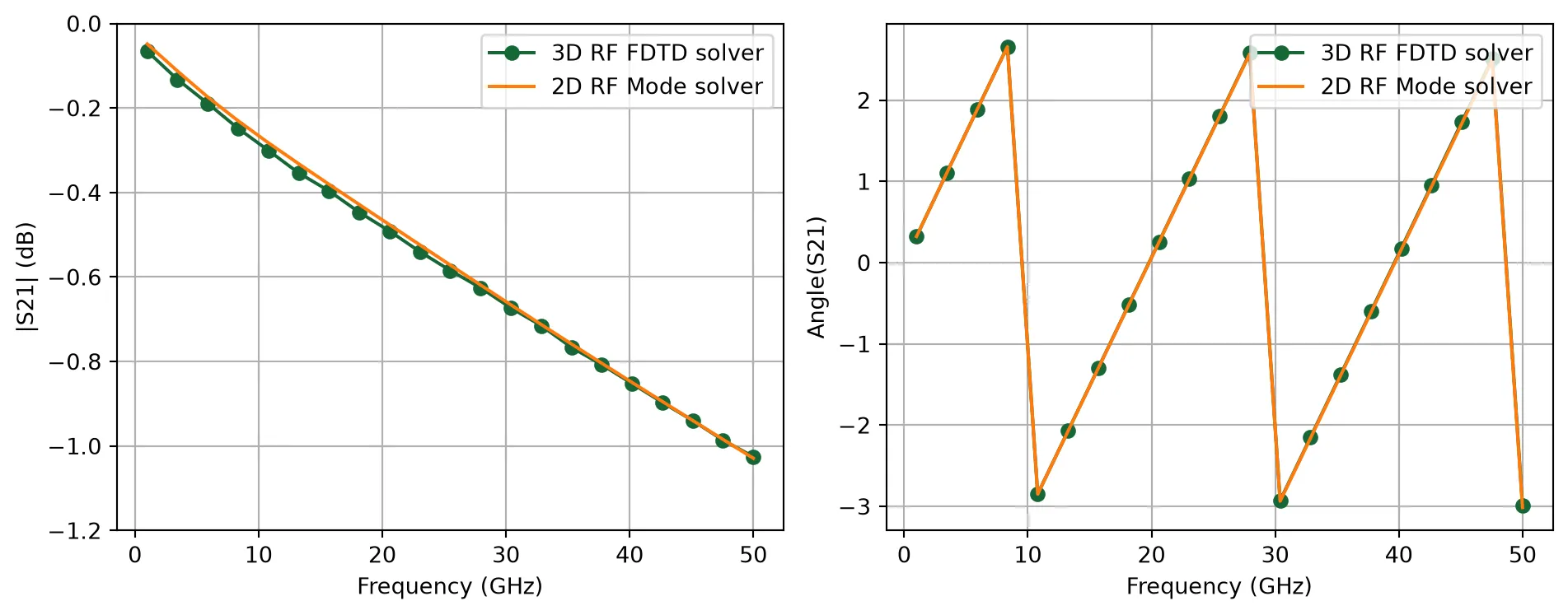
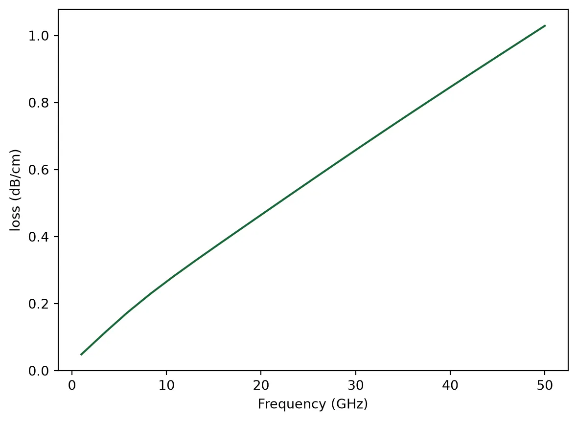
We could also directly use the port_modes data to extract loss.
mode_data = pf.port_modes(dcpw_spec, freqs)# loss in dB/cmalpha = mode_data.data.modes_info["loss (dB/cm)"]
plt.plot(freqs / 1e9, alpha)  # plot loss in dB/cmplt.xlabel("Frequency (GHz)")plt.ylabel("loss (dB/cm)")plt.show()