Optical Fiber

Download notebook (.zip)

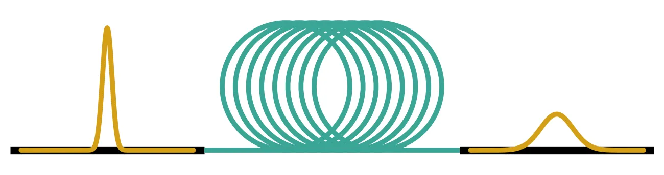
An optical fiber carries light from one chip to another, across a data center or across an ocean. Over these distances, effects that are negligible on a chip shape the signal: the fiber loss, the chromatic dispersion that spreads a pulse because different wavelengths travel at different speeds, the Kerr effect that changes the refractive index with the optical power, and the polarization-mode dispersion (PMD) that delays the two polarizations differently. Long fibers also amplify light by stimulated Raman scattering and can reflect it by stimulated Brillouin scattering.

PhotonForge models all of these. This guide shows how, with standard single-mode fiber at 1550 nm as the example:

Tool	What it models
fiber	Loss, chromatic dispersion and its slope, the Kerr effect, one or two polarizations
pmd_fiber	Polarization-mode dispersion of a randomly birefringent fiber
photonforge.fiber	Unit conversions, split-step section counts, Raman gain and the Brillouin threshold

fiber and pmd_fiber are two-port components with models for both the frequency and the time domain, so they can be placed in a circuit next to the transmitter and receiver chips.

The time-domain fiber runs in the frame that moves with the signal. Light needs about 490 µs to cross 100 km of fiber, which at a 5 ps time step is about 10⁸ samples. The time stepper therefore leaves out the common transit time and keeps everything that changes the shape of the signal. The output appears after a fixed latency, usually hundreds to thousands of samples, set by the length of the dispersion filter, and not after the physical transit time.

import matplotlib.pyplot as plt
import numpy as np
import photonforge as pf
import photonforge.abstract as pfa

# Open the live viewer to display the fiber components
viewer = pf.live_viewer.LiveViewer()

# Use the basic technology for the abstract components
pf.config.default_technology = pf.basic_technology()

# Set the optical carrier at 1550 nm (pf.C_0 is the speed of light in um/s)
f0 = pf.C_0 / 1.55

# Datasheet values of standard single-mode fiber at 1550 nm
smf = pf.fiber.SMF28
print(smf)

LiveViewer started at http://127.0.0.1:46595. Call its 'stop()' method to free the port.
{'attenuation': 0.2, 'dispersion': 17.0, 'dispersion_slope': 0.056, 'effective_area': 80.0, 'kerr_index': 2.6e-20}

Fiber parameters

Fiber datasheets quote the attenuation in dB/km, the dispersion parameter $D$ in ps/(nm km), the dispersion slope $S$ in ps/(nm² km), the effective area $A_\mathrm{eff}$ in µm² and the nonlinear index $n_2$ in m²/W. The propagation constant $\beta(\omega)$ is expanded around the carrier frequency $\omega_0$, and the coefficients that describe propagation follow from the datasheet values [1]:

$$\beta_2 = -\frac{\lambda^2 D}{2\pi c}, \qquad \gamma = \frac{2\pi n_2}{\lambda A_\mathrm{eff}}, \qquad \alpha = \frac{\ln 10}{10}\,\alpha_\mathrm{dB}.$$

Here $\beta_2$ is the group-velocity dispersion, $\gamma$ the nonlinear coefficient and $\alpha$ the power attenuation coefficient. pf.fiber.fiber_parameters performs these conversions and also returns the values in the units used by the PhotonForge models, which is useful when a fiber is modeled directly with an AnalyticWaveguideModel.

# Convert the datasheet values to propagation coefficients
params = pf.fiber.fiber_parameters(**smf)

# Group-velocity dispersion (s²/m)
beta2 = params["beta2"]
# Nonlinear coefficient (1/W/m)
gamma = params["gamma"]
# Power attenuation coefficient (1/m)
alpha = params["alpha"]

print(f"beta2: {beta2 * 1e27:.2f} ps²/km")
print(f"gamma: {gamma * 1e3:.2f} 1/(W km)")
print(f"alpha: {alpha * 1e3:.4f} 1/km")

beta2: -21.68 ps²/km
gamma: 1.32 1/(W km)
alpha: 0.0461 1/km

The values match the ones usually quoted for standard fiber: $\beta_2 \approx -21.7$ ps²/km and $\gamma \approx 1.3$ 1/(W km).

Loss and chromatic dispersion

Without the Kerr effect, the fiber is a linear filter. In the frame moving with the signal, its transfer function at the angular frequency offset $\Omega$ from the carrier is

$$H(\Omega) = \exp\!\left(-\frac{\alpha L}{2}\right) \exp\!\left[i\left(\frac{\beta_2}{2}\Omega^2 + \frac{\beta_3}{6}\Omega^3\right)L\right],$$

where $L$ is the fiber length and $\beta_3$ follows from the dispersion slope. The time stepper applies this response as a finite impulse response (FIR) filter. Its length is set automatically from the spread of delays across the simulation bandwidth, and pf.fiber.filter_taps returns the same value.

A Gaussian pulse with field envelope $\exp[-t^2/(2T_0^2)]$ keeps its Gaussian shape and broadens as [1]

$$T(L) = T_0\sqrt{1 + (L/L_D)^2}, \qquad L_D = \frac{T_0^2}{|\beta_2|},$$

where $L_D$ is the dispersion length. The next cell sends a pulse with $T_0 = 20$ ps through fibers of increasing length, with the loss set to zero so that only the shape changes.

# Create an 80 km fiber with the datasheet values (the defaults of pfa.fiber)
fiber = pfa.fiber(length_km=80.0)
viewer(fiber)

time_step = 2e-12  # Simulation time step (s)
num_steps = 8192  # Number of simulation steps
t0_pulse = 20e-12  # Pulse half-width T0 at 1/e of the field (s)
lengths_km = [10.0, 20.0, 40.0, 80.0]  # Fiber lengths (km)

# Time axis with the pulse centered a quarter of the way into the record
t = (np.arange(num_steps) - num_steps // 4) * time_step

# Gaussian field envelope of the input pulse (sqrt(W))
a_in = np.exp(-0.5 * (t / t0_pulse) ** 2).astype(complex)

# Dispersion length of the pulse (km)
l_dispersion = t0_pulse**2 / abs(beta2) / 1e3
print(f"Dispersion length: {l_dispersion:.1f} km")

# Simulated and closed-form widths for each length
widths, predicted = [], []

fig, ax = plt.subplots(1, 2, figsize=(10, 3.6), tight_layout=True)
ax[0].plot(t * 1e12, np.abs(a_in) ** 2, "k:", label="input")
for length in lengths_km:
    # Create a lossless fiber, so that only the pulse shape changes
    span = pfa.fiber(length_km=length, attenuation=0.0)

    # Time stepper of the fiber
    stepper = span.setup_time_stepper(
        time_step=time_step, carrier_frequency=f0, show_progress=False
    )

    # Run the time stepper on the input field
    a_out = stepper.step(
        inputs=pf.TimeSeries({"P0@0": a_in}, time_step), show_progress=False
    )["P1@0"]

    # Output power (W)
    p_out = np.abs(a_out) ** 2

    # Center of mass of the output pulse, which sits at the filter latency (s)
    t_mean = np.sum(t * p_out) / np.sum(p_out)

    # RMS width of the output power (s)
    t_rms = np.sqrt(np.sum((t - t_mean) ** 2 * p_out) / np.sum(p_out))

    # Width T of the field, sqrt(2) times the RMS width of the power
    widths.append(t_rms * np.sqrt(2))

    # Closed-form width after the same length
    predicted.append(t0_pulse * np.sqrt(1 + (length / l_dispersion) ** 2))

    ax[0].plot((t - t_mean) * 1e12, p_out, label=f"{length:.0f} km")

ax[0].set(xlim=(-250, 250), xlabel="Time (ps)", ylabel="Power (W)")
ax[0].legend()
ax[1].plot(
    lengths_km, np.array(predicted) * 1e12, "k-", label="$T_0\\sqrt{1+(L/L_D)^2}$"
)
ax[1].plot(lengths_km, np.array(widths) * 1e12, "o", label="time stepper")
ax[1].set(xlabel="Fiber length (km)", ylabel="Pulse width $T$ (ps)")
ax[1].legend()
plt.show()

for length, w, p in zip(lengths_km, widths, predicted):
    print(
        f"{length:4.0f} km: simulated {w * 1e12:.2f} ps, closed form {p * 1e12:.2f} ps"
    )

Dispersion length: 18.4 km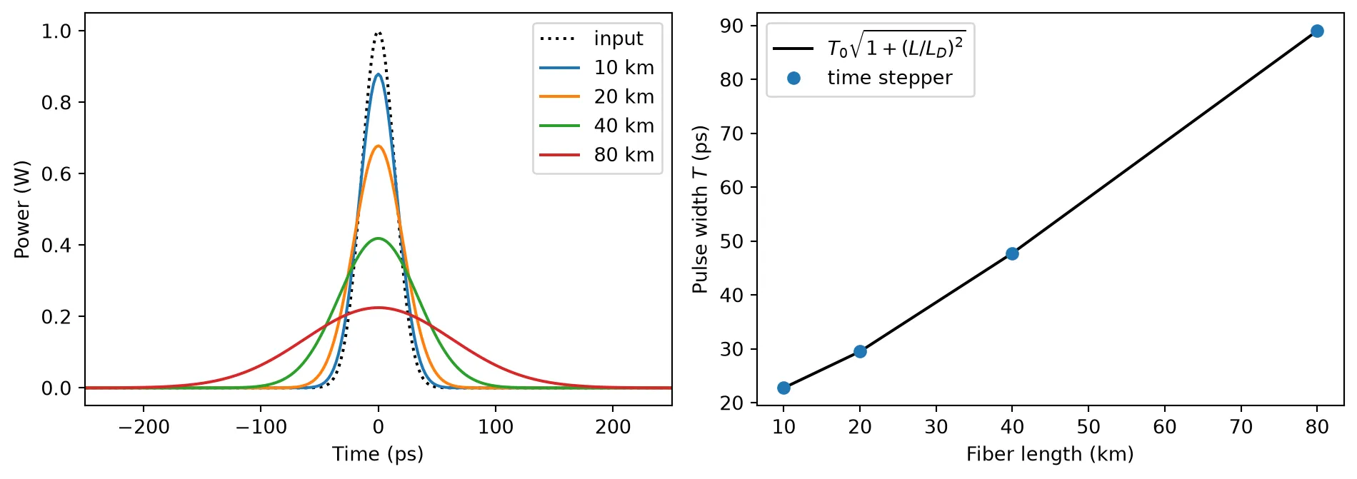

  10 km: simulated 22.75 ps, closed form 22.75 ps
  20 km: simulated 29.50 ps, closed form 29.50 ps
  40 km: simulated 47.76 ps, closed form 47.76 ps
  80 km: simulated 89.01 ps, closed form 89.01 ps

The simulated widths agree with the closed form at every length. The pulse broadens by a factor of 4.5 after 80 km, and its peak power falls by the same factor, since dispersion only redistributes the energy in time.

Dispersion in a short-reach link

Short-reach links in data centers usually detect only the optical power, a scheme called intensity modulation with direct detection (IM/DD). Dispersion limits their reach: the spectral components of each bit travel at different speeds and spill into the neighboring bits. The next cell sends a 25 Gb/s non-return-to-zero (NRZ) signal through 0 km, 10 km and 20 km of fiber at 1550 nm, and through 20 km at 1310 nm, where standard fiber has almost no dispersion. The signal is an ideal, chirp-free intensity modulation, the received signal is the output power $|A|^2$, and no noise is added, so every change in the eye comes from dispersion.

Each eye is characterized by its eye opening, the gap between the lowest one level and the highest zero level at the bit center, divided by the gap between the mean one and zero levels. It is 1 for an undistorted signal and becomes negative when the eye is closed, that is, when some zero bits arrive with more power than some one bits.

The signal is followed by zeros, so that every bit leaves the fiber within the simulated record despite the filter latency.

bit_rate = 25e9  # Bit rate (bit/s)
samples_per_bit = 16  # Number of simulation steps per bit
num_bits = 1024  # Number of transmitted bits
zero_padding = 8192  # Number of zero samples after the signal (steps)
p_one = 1e-3  # Power of a one level (W)

# Simulation time step (s)
dt_eye = 1 / bit_rate / samples_per_bit

# Random number generator for the bits
rng = np.random.default_rng(1)

# Random bit sequence
bits = rng.integers(0, 2, num_bits)

# NRZ waveform with sharp edges, one value per simulation step
p_nrz = np.repeat(bits, samples_per_bit).astype(float)

# Smoothing window half a bit long, which sets the rise time
window = np.hanning(samples_per_bit // 2 + 1)

# Smooth the edges and scale to the one-level power (W)
p_nrz = np.convolve(p_nrz, window / window.sum(), mode="same") * p_one

# Append the zero padding after the last bit
p_nrz = np.concatenate([p_nrz, np.zeros(zero_padding)])

# Chirp-free field: the square root of the power (sqrt(W))
a_nrz = np.sqrt(np.clip(p_nrz, 0, None)).astype(complex)

# Links to compare: (wavelength in um, length in km, dispersion, dispersion slope)
links = [
    (1.55, 1e-3, smf["dispersion"], smf["dispersion_slope"]),
    (1.55, 10.0, smf["dispersion"], smf["dispersion_slope"]),
    (1.55, 20.0, smf["dispersion"], smf["dispersion_slope"]),
    (1.31, 20.0, 0.0, 0.092),
]

fig, ax = plt.subplots(1, len(links), figsize=(13, 3.2), tight_layout=True, sharey=True)
for k, (wavelength, length, dispersion, slope) in enumerate(links):
    # Fiber attenuation at this wavelength (dB/km)
    attenuation = 0.33 if wavelength < 1.4 else smf["attenuation"]

    # Create the fiber at this wavelength
    span = pfa.fiber(
        length_km=length,
        wavelength=wavelength,
        attenuation=attenuation,
        dispersion=dispersion,
        dispersion_slope=slope,
    )

    # Time stepper with the carrier at the fiber's wavelength
    stepper = span.setup_time_stepper(
        time_step=dt_eye, carrier_frequency=pf.C_0 / wavelength, show_progress=False
    )

    # Run the time stepper on the input field
    a_out = stepper.step(
        inputs=pf.TimeSeries({"P0@0": a_nrz}, dt_eye), show_progress=False
    )["P1@0"]

    # Filter latency of the single-section fiber, in samples
    latency = (
        pf.fiber.filter_taps(
            length,
            dt_eye,
            wavelength=wavelength,
            dispersion=dispersion,
            dispersion_slope=slope,
        )
        // 2
    )

    # Received power, aligned with the transmitted bits
    p_rx = np.abs(np.roll(a_out, -latency)) ** 2

    # Received power at each bit center
    centers = p_rx[samples_per_bit // 2 : num_bits * samples_per_bit : samples_per_bit]

    # Received power of the one bits
    ones = centers[bits == 1]

    # Received power of the zero bits
    zeros = centers[bits == 0]

    # Eye opening at the bit center
    opening = (ones.min() - zeros.max()) / (ones.mean() - zeros.mean())
    print(f"{wavelength * 1e3:.0f} nm, {length:4.1f} km: eye opening {opening:+.2f}")

    # Cut the received power into one-bit traces
    traces = p_rx[: num_bits * samples_per_bit].reshape(-1, samples_per_bit)

    # Join consecutive traces into 2-bit windows to draw the eye
    traces = np.hstack([traces[:-1], traces[1:]])

    # Time axis of the eye (ps)
    t_eye = np.arange(2 * samples_per_bit) * dt_eye * 1e12
    ax[k].plot(t_eye, traces[2:300].T * 1e3, color="tab:blue", alpha=0.08)
    ax[k].set(
        title=f"{wavelength * 1e3:.0f} nm, {length:.0f} km, opening {opening:+.2f}",
        xlabel="Time (ps)",
    )
ax[0].set_ylabel("Received power (mW)")
plt.show()

1550 nm,  0.0 km: eye opening +1.00
1550 nm, 10.0 km: eye opening +0.66
1550 nm, 20.0 km: eye opening -0.08
1310 nm, 20.0 km: eye opening +1.00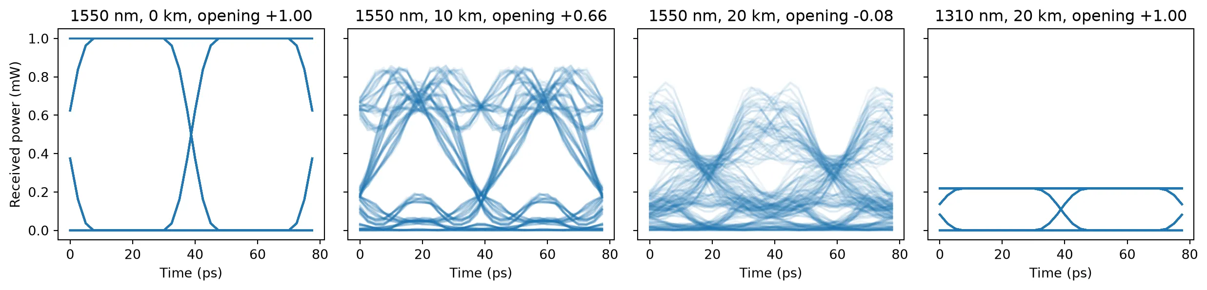

At 1550 nm the eye closes with distance: the eye opening falls from 1.00 at the transmitter to 0.66 after 10 km, and turns negative after 20 km. Dispersion turns the spread of arrival times into power ripples, so some one levels overshoot and the zero levels rise between ones. The reach scales as $1/B^2$ with the bit rate $B$, so at 50 Gb/s the eye already closes after about 5 km. The same 20 km of fiber at 1310 nm keeps the eye open, at a lower power because of the higher loss, since the dispersion of standard fiber is close to zero there. This is why short-reach IM/DD links, which cannot undo dispersion at the receiver, run in the O-band around 1310 nm. Coherent links instead detect the optical field and remove dispersion in digital signal processing, as shown in Dual-polarization link below.

Kerr nonlinearity and the split-step method

The Kerr effect adds $\Delta n = n_2 P/A_\mathrm{eff}$ to the refractive index, so a pulse modulates its own phase. This self-phase modulation (SPM) gives the field a phase proportional to the instantaneous power, $\phi_\mathrm{NL}(t) = \gamma P(t) L_\mathrm{eff}$, where the effective length $L_\mathrm{eff} = (1 - e^{-\alpha L})/\alpha$ accounts for the power lost along the fiber.

The Kerr effect and dispersion act together along the fiber, and the time stepper treats them with the split-step method: the fiber is divided into sections, and each section applies the nonlinear phase and then the dispersion. pfa.fiber chooses the number of sections from peak_power, the largest power the signal will reach, so that the nonlinear phase per section stays below max_phase (0.05 rad by default). A linear fiber, with peak_power=0, is a single section. pf.fiber.section_count returns the same number before the fiber is built.

Self-phase modulation

Without dispersion, SPM leaves the pulse shape unchanged and broadens its spectrum. Two instants on the pulse with the same rate of phase change give the same frequency, and their contributions interfere, so the spectrum develops a set of peaks. For a peak phase $\phi_\mathrm{max}$, the number of peaks $M$ follows $\phi_\mathrm{max} \approx (M - \tfrac{1}{2})\pi$ [1]. The next cell sets the launch power for $\phi_\mathrm{max} = 1.5\pi$, $2.5\pi$ and $3.5\pi$ in 25 km of fiber, with the dispersion set to zero.

dt_spm = 1e-12  # Simulation time step (s)
n_spm = 32768  # Number of simulation steps
t0_spm = 50e-12  # Pulse half-width T0 at 1/e of the field (s)
length_spm = 25.0  # Fiber length (km)
phi_targets = [1.5, 2.5, 3.5]  # Peak nonlinear phases, in units of pi

# Time axis centered on the pulse
t_spm = (np.arange(n_spm) - n_spm // 2) * dt_spm

# Frequency axis of the spectrum (Hz), sign flipped for the envelope convention
nu = -np.fft.fftshift(np.fft.fftfreq(n_spm, dt_spm))

# Effective length of the fiber (m)
l_eff = (1 - np.exp(-alpha * length_spm * 1e3)) / alpha

fig, ax = plt.subplots(1, 3, figsize=(12, 3.2), tight_layout=True)
for k, phi in enumerate(phi_targets):
    # Peak power that gives this nonlinear phase (W)
    p_peak = phi * np.pi / (gamma * l_eff)

    # Create the fiber without dispersion, sectioned for this peak power
    span = pfa.fiber(
        length_km=length_spm, peak_power=p_peak, dispersion=0.0, dispersion_slope=0.0
    )

    # Time stepper of the fiber
    stepper = span.setup_time_stepper(
        time_step=dt_spm, carrier_frequency=f0, show_progress=False
    )

    # Gaussian input field with this peak power (sqrt(W))
    a_in = np.sqrt(p_peak) * np.exp(-0.5 * (t_spm / t0_spm) ** 2).astype(complex)

    # Run the time stepper on the input field
    a_out = stepper.step(
        inputs=pf.TimeSeries({"P0@0": a_in}, dt_spm), show_progress=False
    )["P1@0"]

    # Power spectrum of the output field
    spectrum = np.abs(np.fft.fftshift(np.fft.fft(a_out))) ** 2

    # Keep the central +-30 GHz of the spectrum
    keep = np.abs(nu) < 30e9

    # Spectrum normalized to its maximum
    s = spectrum[keep] / spectrum[keep].max()

    # Count the local maxima above 2% of the maximum
    peaks = np.sum((s[1:-1] > s[:-2]) & (s[1:-1] >= s[2:]) & (s[1:-1] > 0.02))

    print(
        f"phi_max = {phi} pi: peak power {p_peak * 1e3:.0f} mW, "
        f"{len(span.references)} sections, {peaks} spectral peaks"
    )
    ax[k].plot(nu[keep] / 1e9, s)
    ax[k].set(
        title=f"$\\phi_{{max}}$ = {phi}$\\pi$, {peaks} peaks", xlabel="Frequency (GHz)"
    )
ax[0].set_ylabel("Normalized spectrum")
plt.show()

phi_max = 1.5 pi: peak power 241 mW, 0 sections, 2 spectral peaks
phi_max = 2.5 pi: peak power 402 mW, 0 sections, 3 spectral peaks
phi_max = 3.5 pi: peak power 562 mW, 0 sections, 4 spectral peaks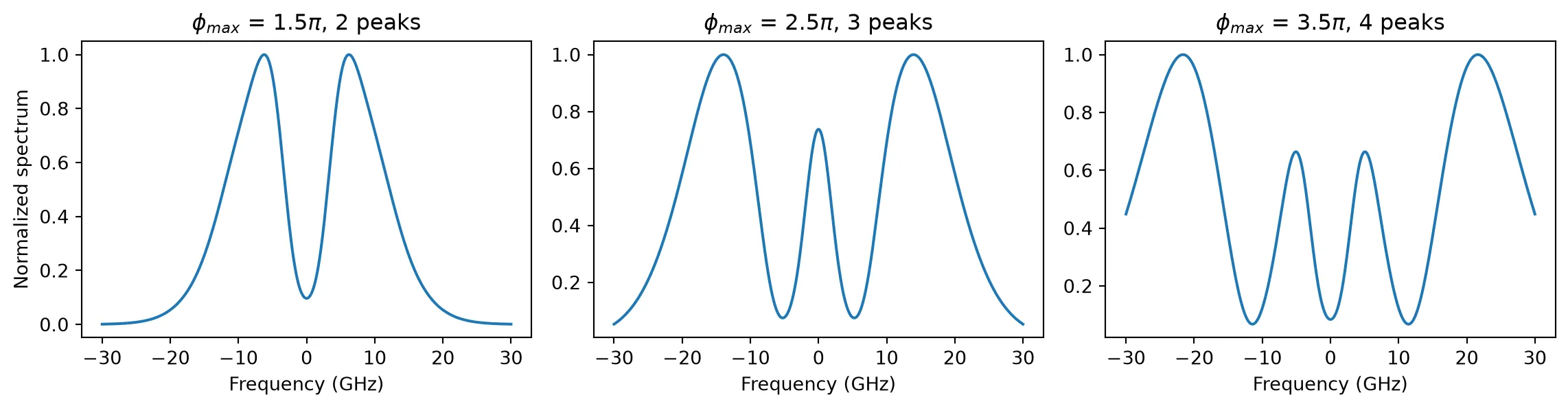

The spectra show exactly 2, 3 and 4 peaks, as the rule predicts. The fibers are split into 159, 265 and 371 sections, because the peak power reaches hundreds of milliwatts while each section is limited to 0.05 rad of nonlinear phase. Since the dispersion is zero here, every section is a simple phase rotation and the run takes a few seconds.

The fundamental soliton

In the anomalous dispersion regime ($\beta_2 < 0$, the case of standard fiber at 1550 nm), SPM and dispersion can balance. A hyperbolic-secant pulse $\sqrt{P_0}\,\mathrm{sech}(t/T_0)$ with the peak power

$$P_0 = \frac{|\beta_2|}{\gamma T_0^2}$$

propagates without changing shape in a lossless fiber. It is the fundamental soliton [1]. The next cell sends a soliton with $T_0 = 20$ ps through one dispersion length, 18.4 km, and compares it with the same pulse in a fiber without the Kerr effect, and in a fiber with the normal 0.2 dB/km of loss.

dt_sol = 2e-12  # Simulation time step (s)
n_sol = 20000  # Number of simulation steps

# Time axis centered on the pulse
t_sol = (np.arange(n_sol) - n_sol // 2) * dt_sol

# Soliton peak power for T0 = 20 ps (W)
p_soliton = abs(beta2) / (gamma * t0_pulse**2)
print(f"Soliton peak power: {p_soliton * 1e3:.1f} mW")

# Hyperbolic-secant input field (sqrt(W))
a_sech = np.sqrt(p_soliton) / np.cosh(np.clip(t_sol / t0_pulse, -300, 300))

# Convert the input field to complex values
a_sech = a_sech.astype(complex)

# Fiber variants: (label, nonlinear index, attenuation in dB/km)
variants = [
    ("dispersion only", 0.0, 0.0),
    ("soliton, lossless", smf["kerr_index"], 0.0),
    ("soliton, 0.2 dB/km", smf["kerr_index"], 0.2),
]

fig, ax = plt.subplots(figsize=(6.5, 3.6), tight_layout=True)
ax.plot(t_sol * 1e12, np.abs(a_sech) ** 2 / p_soliton, "k:", label="input")
for label, kerr_index, attenuation in variants:
    # Create one dispersion length of fiber, sectioned for the soliton power
    span = pfa.fiber(
        length_km=l_dispersion,
        peak_power=p_soliton,
        kerr_index=kerr_index,
        attenuation=attenuation,
    )

    # Time stepper of the fiber
    stepper = span.setup_time_stepper(
        time_step=dt_sol, carrier_frequency=f0, show_progress=False
    )

    # Run the time stepper on the input field
    a_out = stepper.step(
        inputs=pf.TimeSeries({"P0@0": a_sech}, dt_sol), show_progress=False
    )["P1@0"]

    # Output power (W)
    p_out = np.abs(a_out) ** 2

    # Times at which the output power is above half its maximum (s)
    above = t_sol[p_out > p_out.max() / 2]

    # Full width at half maximum of the output (s)
    fwhm = above[-1] - above[0]
    print(f"{label}: FWHM {fwhm * 1e12:.1f} ps")

    # Time of the output peak, used to center the plot (s)
    t_peak = t_sol[np.argmax(p_out)]
    ax.plot((t_sol - t_peak) * 1e12, p_out / p_soliton, label=label)

# Width of the input, measured on the same time grid as the outputs (s)
above = t_sol[np.abs(a_sech) ** 2 > p_soliton / 2]
print(f"Input FWHM on the time grid: {(above[-1] - above[0]) * 1e12:.1f} ps")
ax.set(xlim=(-120, 120), xlabel="Time (ps)", ylabel="Power / $P_0$")
ax.legend()
plt.show()

Soliton peak power: 41.1 mW
dispersion only: FWHM 52.0 ps
soliton, lossless: FWHM 32.0 ps
soliton, 0.2 dB/km: FWHM 40.0 ps
Input FWHM on the time grid: 32.0 ps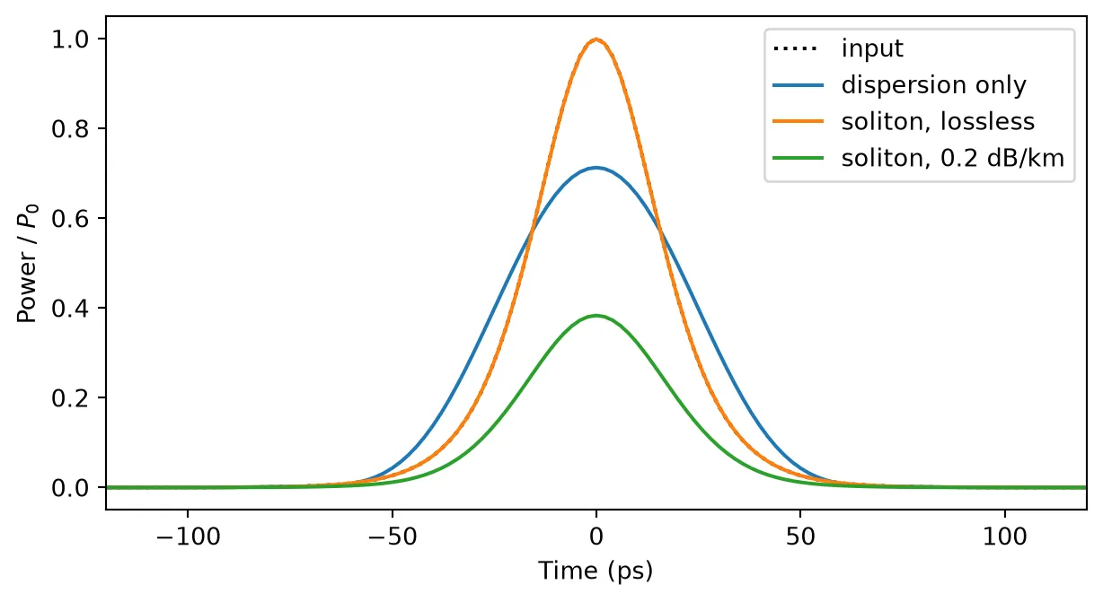

The widths are full widths at half maximum (FWHM), measured on the 2 ps time grid of the simulation, which gives 32 ps for the input (35.3 ps exactly). Dispersion alone broadens the pulse to 52 ps. With the Kerr effect at the soliton power the width stays at 32 ps, and the output overlaps the input in the plot. With the fiber loss, the power falls along the fiber, the balance is lost, and the pulse broadens to 40 ps.

Polarization-mode dispersion

A real fiber is slightly birefringent, so its two polarizations travel at slightly different speeds, and the birefringent axes rotate randomly along its length. The fiber as a whole is then described by a 2 × 2 Jones matrix $J(\omega)$ that maps the two input polarizations to the two output polarizations. Because PMD causes no loss, $J$ is unitary at every frequency.

At each frequency, two input polarizations, the principal states of polarization, reach the output without changing their polarization to first order in frequency. Their delays differ by the differential group delay (DGD) $\Delta\tau$. The DGD of a fiber is a random quantity: over many fibers, or over time on one fiber, it follows a Maxwellian distribution whose mean grows with the square root of length [3],

$$\langle \Delta\tau \rangle = D_\mathrm{PMD}\sqrt{L},$$

where the PMD coefficient $D_\mathrm{PMD}$ is about 0.1 ps/√km for modern fiber and 0.5 ps/√km or more for older installed cable.

pfa.pmd_fiber returns a two-port component whose ports carry two modes, one per polarization. Its PolarizationModeDispersionModel builds $J(\omega)$ with the coarse-step method: the fiber is divided into segments birefringent sections separated by random rotations. Each seed selects one fiber; the same seed always gives the same fiber. The model’s differential_group_delay method extracts the DGD from the Jones matrix the same way a commercial PMD analyzer does.

pmd_coefficient = 0.1  # PMD coefficient (ps/sqrt(km))
length_pmd = 80.0  # Fiber length (km)

# Create one 80 km fiber realization and display it
pmd_span = pfa.pmd_fiber(length_km=length_pmd, pmd=pmd_coefficient, seed=3)
viewer(pmd_span)

# Frequencies across 2 THz around the carrier (Hz)
freqs = f0 + np.linspace(-1e12, 1e12, 401)

# DGD of this fiber at each frequency (s)
dgd_freq = pmd_span.active_model.differential_group_delay(freqs)

# DGD at the carrier of 2000 different fibers (s)
dgd_fibers = np.array(
    [
        pf.PolarizationModeDispersionModel(
            length_km=length_pmd, pmd=pmd_coefficient, segments=60, seed=seed
        ).differential_group_delay([f0])[0]
        for seed in range(2000)
    ]
)

# Scale of the Maxwellian with the same RMS value as the 2000 fibers (s)
sigma = np.sqrt(np.mean(dgd_fibers**2) / 3)

# DGD axis of the Maxwellian (s)
x = np.linspace(0, dgd_fibers.max(), 300)

# Maxwellian probability density (1/s)
maxwell = np.sqrt(2 / np.pi) * x**2 / sigma**3 * np.exp(-(x**2) / (2 * sigma**2))

fig, ax = plt.subplots(1, 2, figsize=(11, 3.6), tight_layout=True)
ax[0].plot((freqs - f0) / 1e12, dgd_freq * 1e12)
ax[0].axhline(
    pmd_coefficient * np.sqrt(length_pmd), color="gray", ls="--", label="mean"
)
ax[0].set(xlabel="Frequency offset (THz)", ylabel="DGD (ps)", title="One fiber")
ax[0].legend()
ax[1].hist(dgd_fibers * 1e12, bins=40, density=True, alpha=0.6, label="2000 fibers")
ax[1].plot(x * 1e12, maxwell / 1e12, "k", label="Maxwellian")
ax[1].set(
    xlabel="DGD (ps)", ylabel="Probability density (1/ps)", title="At the carrier"
)
ax[1].legend()
plt.show()

print(f"Mean DGD over 2000 fibers: {dgd_fibers.mean() * 1e12:.3f} ps")
print(f"D_PMD sqrt(L): {pmd_coefficient * np.sqrt(length_pmd):.3f} ps")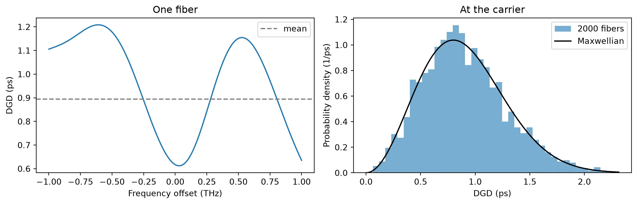

Mean DGD over 2000 fibers: 0.902 ps
D_PMD sqrt(L): 0.894 ps

The left plot shows that the DGD of a single fiber varies with frequency, here between 0.6 ps and 1.2 ps across 2 THz. The right plot shows the DGD at one frequency over 2000 fibers: it follows the Maxwellian distribution, with a mean of 0.90 ps against $D_\mathrm{PMD}\sqrt{L} = 0.89$ ps.

Pulse splitting in the time domain

In the time domain, the pmd_fiber component uses PolarizationModeDispersionTimeStepper, which applies the Jones matrix of the same fiber as a 2 × 2 FIR filter. A pulse launched in one principal state leaves the fiber as a single pulse. A pulse whose power is split equally between the two principal states leaves as two copies, one in each output principal state, separated by the DGD. This picture holds when the signal bandwidth is small compared with the frequency range over which the DGD stays constant, roughly $1/\Delta\tau$.

The next cell uses an old 100 km fiber with $D_\mathrm{PMD} = 1$ ps/√km and a pulse with 25 ps FWHM. The principal states follow from the Jones matrix at two close frequencies, $J_1$ at $f_0$ and $J_2$ at $f_0 + \delta f$: the input principal states are the eigenvectors of $J_1^{-1}J_2$ and the output principal states are the eigenvectors of $J_2 J_1^{-1}$. The Jones matrix is read from the component’s S matrix, whose element from P0@i to P1@j is $J_{ji}$.

length_old = 100.0  # Fiber length (km)
pmd_old = 1.0  # PMD coefficient of old installed fiber (ps/sqrt(km))
delta_f = 1e9  # Frequency step for the principal states (Hz)

# Create one realization of the old fiber
old_span = pfa.pmd_fiber(length_km=length_old, pmd=pmd_old, seed=5)

# S matrix of the fiber at the carrier and at a close frequency
s_matrix = old_span.s_matrix([f0, f0 + delta_f], show_progress=False)

# Jones matrices at the two frequencies
jones = np.zeros((2, 2, 2), dtype=complex)
for i in range(2):
    for j in range(2):
        # Transmission from input mode i to output mode j
        jones[:, j, i] = s_matrix[(f"P0@{i}", f"P1@{j}")]

# Input principal states, the eigenvectors of J1^-1 J2 (as columns)
_, psp_in = np.linalg.eig(np.linalg.inv(jones[0]) @ jones[1])

# Output principal states, the eigenvectors of J2 J1^-1 (as columns)
_, psp_out = np.linalg.eig(jones[1] @ np.linalg.inv(jones[0]))

# DGD of this fiber at the carrier (s)
dgd = old_span.active_model.differential_group_delay([f0])[0]
print(f"DGD at the carrier: {dgd * 1e12:.2f} ps")

DGD at the carrier: 11.02 ps

dt_pmd = 1e-12  # Simulation time step (s)
n_pmd = 2000  # Number of simulation steps
fwhm_pmd = 25e-12  # Pulse FWHM (s)
t_launch = 300e-12  # Time of the pulse center at the input (s)

# Time axis (s)
t_pmd = np.arange(n_pmd) * dt_pmd

# Gaussian input envelope (sqrt(W))
envelope = np.exp(-2 * np.log(2) * ((t_pmd - t_launch) / fwhm_pmd) ** 2).astype(complex)

# Input polarizations: one principal state, and an equal split between both
launches = {
    "one principal state": psp_in[:, 0],
    "equal split": (psp_in[:, 0] + psp_in[:, 1]) / np.sqrt(2),
}

# Time stepper of the old fiber
stepper = old_span.setup_time_stepper(
    time_step=dt_pmd, carrier_frequency=f0, show_progress=False
)

fig, ax = plt.subplots(1, 2, figsize=(11, 3.6), tight_layout=True, sharey=True)
for k, (label, polarization) in enumerate(launches.items()):
    # Reset the stepper's filter history before each run
    stepper.reset()

    # Input field on the two modes, with this polarization
    inputs = {"P0@0": polarization[0] * envelope, "P0@1": polarization[1] * envelope}

    # Run the time stepper on the pulse
    outputs = stepper.step(inputs=pf.TimeSeries(inputs, dt_pmd), show_progress=False)

    # Output field on the two modes
    field = np.array([outputs["P1@0"], outputs["P1@1"]])

    for m in range(2):
        # Power in each output principal state
        p_state = np.abs(np.conj(psp_out[:, m]) @ field) ** 2

        # Arrival time of this component, as its center of mass (s)
        t_arrival = np.sum(t_pmd * p_state) / max(np.sum(p_state), 1e-30)

        # Share of the output power in this state
        share = p_state.sum() / np.sum(np.abs(field) ** 2)
        print(
            f"{label}, output state {m}: {share:.3f} of the power, "
            f"at {t_arrival * 1e12:.1f} ps"
        )
        ax[k].plot(t_pmd * 1e12, p_state, label=f"output principal state {m}")
    ax[k].set(title=f"Launch in {label}", xlabel="Time (ps)", xlim=(700, 920))
    ax[k].legend()
ax[0].set_ylabel("Power (W)")
plt.show()

one principal state, output state 0: 0.001 of the power, at 809.4 ps
one principal state, output state 1: 0.999 of the power, at 817.4 ps
equal split, output state 0: 0.506 of the power, at 806.8 ps
equal split, output state 1: 0.494 of the power, at 817.5 ps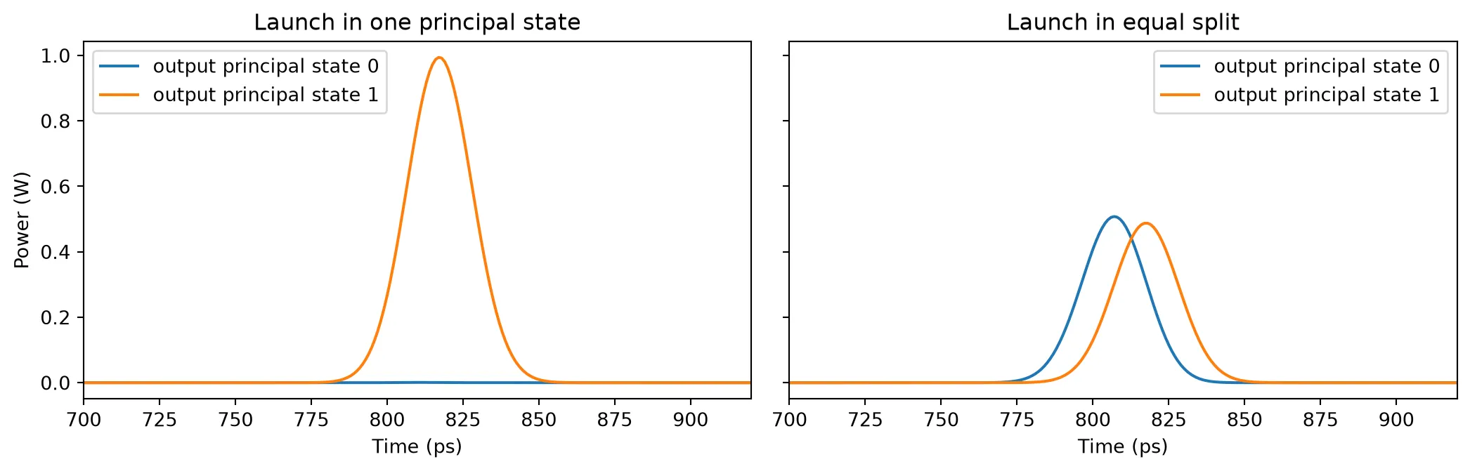

Launched in one principal state, 99.9% of the power leaves the fiber in a single output principal state and the pulse keeps its shape. Split equally, the power leaves in both output states, about half in each, and the two copies arrive 10.7 ps apart, close to the DGD of 11.0 ps. The output appears after about 810 ps rather than the 300 ps of the input, because the FIR filter adds a fixed latency of half its length. In a link, the receiver sees the sum of the two copies, a pulse broadened by the DGD.

Dual-polarization link

Coherent transceivers send independent data on the two polarizations, which doubles the capacity of the fiber. With dual_polarization=True, pfa.fiber has two modes per port, one per polarization. Loss and dispersion act on both alike, so the dual-polarization fiber connects directly to pmd_fiber, and the pair forms a complete linear span.

For the Kerr effect, a fiber with random birefringence averages the nonlinear coupling between the two polarizations, and the nonlinear phase becomes $\tfrac{8}{9}\gamma P$, where $P$ is the total power in both polarizations [4]. With dual_polarization=True, pfa.fiber applies this factor.

The next cells send a dual-polarization quadrature phase-shift keying (DP-QPSK) signal at 32 GBd through 80 km of standard fiber. Its PMD is that of older cable ($D_\mathrm{PMD} = 0.5$ ps/√km), added by a pmd_fiber of the same length. A coherent receiver measures the optical field of both polarizations. Here the receiver is ideal: it reads the output field of the span directly.

baud_rate = 32e9  # Symbol rate (symbol/s)
samples_per_symbol = 8  # Number of simulation steps per symbol
num_symbols = 2048  # Number of transmitted symbols per polarization
zero_padding = 4096  # Number of zero samples after the signal (steps)
p_launch = 1e-3  # Launch power, both polarizations together (W)
length_link = 80.0  # Fiber length (km)
pmd_link = 0.5  # PMD coefficient (ps/sqrt(km))

# Simulation time step (s)
dt_link = 1 / baud_rate / samples_per_symbol

# Total number of simulation steps, including the padding
n_link = num_symbols * samples_per_symbol + zero_padding

# Random number generator for the symbols
rng = np.random.default_rng(3)

# Random QPSK symbols for each polarization
symbols = rng.choice([-1, 1], (2, num_symbols)) + 1j * rng.choice(
    [-1, 1], (2, num_symbols)
)

# Normalize the symbols to unit average power
symbols /= np.sqrt(2)

# Time axis of the pulse, four symbols on each side of its center (s)
t_pulse = np.arange(-4 * samples_per_symbol, 4 * samples_per_symbol + 1) * dt_link

# Gaussian pulse whose power has a FWHM of half a symbol
pulse = np.exp(-2 * np.log(2) * (t_pulse * 2 * baud_rate) ** 2)

# Empty field of both polarizations, including the padding
tx = np.zeros((2, n_link), dtype=complex)

# Place each symbol at the center of its slot
tx[
    :, samples_per_symbol // 2 : num_symbols * samples_per_symbol : samples_per_symbol
] = symbols

# Shape the symbols with the pulse, half the launch power per polarization (sqrt(W))
tx = np.array([np.convolve(pol, pulse, mode="same") for pol in tx]) * np.sqrt(
    p_launch / 2
)

# Create the span component
link = pf.Component("DP span")

# Add the dual-polarization fiber
fiber_ref = link.add_reference(pfa.fiber(length_km=length_link, dual_polarization=True))

# Add the PMD of the same length of old cable
pmd_ref = link.add_reference(pfa.pmd_fiber(length_km=length_link, pmd=pmd_link, seed=2))

# Connect the PMD section after the fiber
pmd_ref.connect("P0", fiber_ref["P1"])

# Expose the fiber's input as the span's input port
link.add_port(fiber_ref["P0"], "P0")

# Expose the PMD section's output as the span's output port
link.add_port(pmd_ref["P1"], "P1")

# Add a circuit model to simulate the span
link.add_model(pf.CircuitModel(), "Circuit")
viewer(link)

LayoutSchematic

# Circuit time stepper of the span
stepper = link.setup_time_stepper(
    time_step=dt_link, carrier_frequency=f0, show_progress=False
)

# Run it on both polarizations
outputs = stepper.step(
    inputs=pf.TimeSeries({"P0@0": tx[0], "P0@1": tx[1]}, dt_link), show_progress=False
)

# Received field on the two output modes
rx = np.array([outputs["P1@0"], outputs["P1@1"]])

Recovering the data

A coherent receiver undoes the channel in digital signal processing [5]. It first removes the chromatic dispersion, which is the same for both polarizations and known from the fiber length. It then undoes the polarization rotation and the PMD with a 2 × 2 multiple-input multiple-output (MIMO) equalizer, which mixes the two received polarizations back into the two transmitted ones. Real receivers estimate this 2 × 2 response adaptively from the signal. Here both steps use the frequency response of the components themselves:

• The dispersion response $H_\mathrm{CD}(\Omega)$ is the S matrix of the fiber from P0@0 to P1@0.
• The full response $H(\Omega)$ of the span is the 2 × 2 S matrix of the circuit.

Dividing by $H_\mathrm{CD}$ removes the dispersion only, and multiplying by $H^{-1}$ removes the whole channel. The S matrices are evaluated at $f_0 - \nu$ for each frequency $\nu$ of the discrete Fourier transform, because a component $e^{+i 2\pi \nu t}$ of the field envelope sits at the physical frequency $f_0 - \nu$. The FIR filters delay the output by a whole number of samples, which the receiver finds by correlating the result with the known transmitted signal, as it would with a training sequence. The quality of the recovered symbols is measured by the error vector magnitude (EVM), the RMS distance between received and transmitted symbols relative to the RMS symbol amplitude.

# Frequencies of the discrete Fourier transform (Hz)
nu = np.fft.fftfreq(n_link, dt_link)

# S matrix of the fiber alone
s_fiber = fiber_ref.component.s_matrix(f0 - nu, show_progress=False)

# Dispersion response, the same for both polarizations
h_cd = s_fiber[("P0@0", "P1@0")]

# S matrix of the whole span
s_link = link.s_matrix(f0 - nu, show_progress=False)

# 2x2 response of the span at each frequency
h_link = np.zeros((n_link, 2, 2), dtype=complex)
for i in range(2):
    for j in range(2):
        # Transmission from input mode i to output mode j
        h_link[:, j, i] = s_link[(f"P0@{i}", f"P1@{j}")]

# Received spectrum of each polarization
rx_spectrum = np.fft.fft(rx, axis=1)

# Receiver outputs: no processing, dispersion removed, whole channel removed
equalized = {
    "received": rx,
    "dispersion removed": np.fft.ifft(rx_spectrum / h_cd, axis=1),
    "dispersion and PMD removed": np.fft.ifft(
        np.einsum("nij,jn->in", np.linalg.inv(h_link), rx_spectrum), axis=1
    ),
}

# Sample index of each symbol center
centers = samples_per_symbol // 2 + samples_per_symbol * np.arange(num_symbols)

# Transmitted samples at the symbol centers, normalized to the launch amplitude
tx_samples = tx[:, centers] / np.sqrt(p_launch / 2)

# EVM of the transmitted signal itself, from the overlap of neighboring pulses
evm_tx = np.sqrt(np.mean(np.abs(tx_samples - symbols) ** 2))
print(f"transmitted: EVM {evm_tx * 100:.2f}%")

fig, ax = plt.subplots(2, 3, figsize=(11, 7), tight_layout=True)
for k, (label, signal) in enumerate(equalized.items()):
    # Correlation of the result with the transmitted X polarization
    corr = np.fft.ifft(np.fft.fft(signal[0]) * np.conj(np.fft.fft(tx[0])))

    # Delay of the result, at the correlation peak (steps)
    delay = int(np.argmax(np.abs(corr)))

    # Remove the delay and keep the samples at the symbol centers
    samples = np.roll(signal, -delay, axis=1)[:, centers]

    # Normalize to the launch amplitude of each polarization
    samples /= np.sqrt(p_launch / 2)

    # Error vector magnitude against the transmitted symbols, after equalization
    evm = np.sqrt(
        np.mean(np.abs(samples - symbols) ** 2) / np.mean(np.abs(symbols) ** 2)
    )
    if label != "received":
        print(f"{label}: delay {delay} steps, EVM {evm * 100:.2f}%")

    for m, name in enumerate(["X", "Y"]):
        # Scale each constellation by its RMS amplitude for display
        shown = samples[m] / np.sqrt(np.mean(np.abs(samples[m]) ** 2))
        ax[m, k].plot(shown.real, shown.imag, ".", ms=2)
        ax[m, k].set(
            title=f"{name}: {label}", aspect="equal", xlim=(-2, 2), ylim=(-2, 2)
        )
plt.show()

transmitted: EVM 0.55%
dispersion removed: delay 1087 steps, EVM 119.11%
dispersion and PMD removed: delay 1088 steps, EVM 0.55%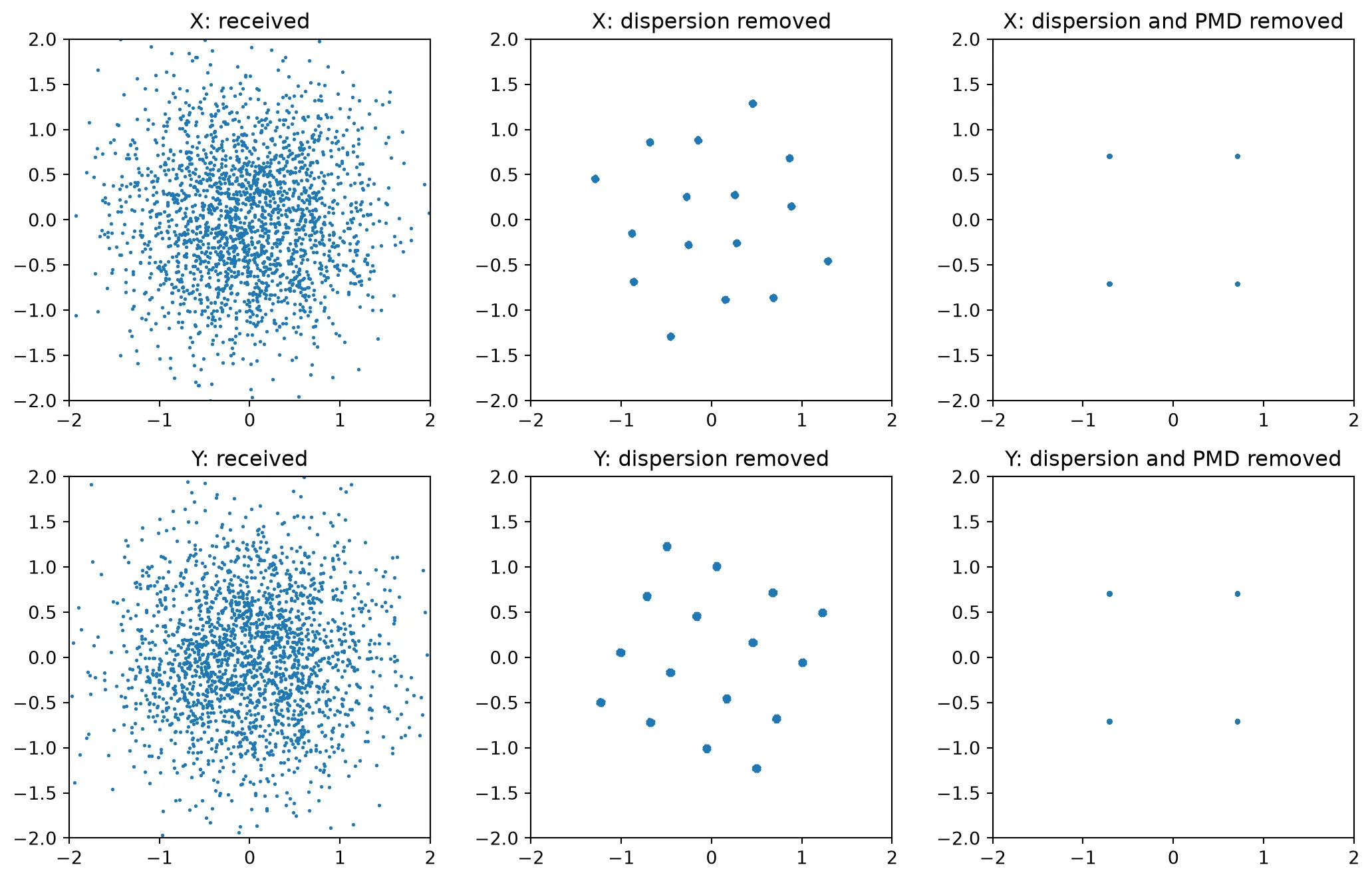

The received symbols form a cloud: after 80 km, dispersion spreads each symbol over many symbol periods. Removing the dispersion leaves the PMD. Its main effect here is the random rotation of the polarization, so each received polarization carries a fixed mixture of the X and Y symbols, and the constellation shows the 16 combinations of two QPSK symbols. Removing the whole channel recovers both QPSK constellations with an EVM of 0.55%. The transmitted signal already has this EVM: neighboring Gaussian pulses overlap slightly at each symbol center. The equalized signal is therefore identical to the transmitted signal, and the dispersion-removed signal, at 119% EVM, shows how far the polarization mixing alone moves the symbols.

The time-domain simulation and the frequency-domain S matrices describe the same span: the inverse of the circuit’s S matrix undoes the output of the circuit’s time stepper.

Raman gain and the Brillouin threshold

Two further effects scatter light off vibrations of the glass, and both depend on the power and length of the fiber rather than on the signal waveform.

Stimulated Raman scattering transfers power from a pump to light about 13 THz lower in frequency. A strong pump at 1450 nm therefore amplifies a 1550 nm signal along the whole fiber, which is the basis of distributed Raman amplifiers. With an undepleted pump, the on/off gain, the signal gain with the pump on relative to the pump off, is [2]

$$G_\mathrm{on/off} = \exp\!\left(C_R P_p L_\mathrm{eff,p}\right),$$

where $C_R$ is the Raman gain efficiency in 1/(W km), $P_p$ the pump power and $L_\mathrm{eff,p}$ the effective length at the pump wavelength. pf.fiber.raman_on_off_gain evaluates this closed form, and pf.fiber.raman_profile solves the coupled power equations of pump and signal along the fiber, including pump depletion, for a pump launched with the signal (co-pumping) or from the far end (counter-pumping).

Stimulated Brillouin scattering reflects light back toward the transmitter, shifted down by about 11 GHz. Its gain is very high but only 20 MHz wide, so it limits the power of narrow-linewidth light. pf.fiber.brillouin_threshold returns the input power at which the backscattered power grows to the level of the transmitted power, following Smith’s estimate [6]. A source broader than the Brillouin gain bandwidth spreads its power over many gain windows, which raises the threshold by the ratio of the two widths.

length_raman = 80.0  # Fiber length (km)
p_signal = 1e-3  # Signal power at the input (W)
pump_powers = np.linspace(0.0, 0.5, 26)  # Pump powers (W)

# Frequency shifts between pump and signal (Hz)
shift = np.linspace(0.1e12, 35e12, 1000)

# Raman gain efficiency at each shift (1/(W km))
efficiency = pf.fiber.raman_efficiency_at_shift(shift)

# On/off gain from the closed form, for each pump power (dB)
gain_closed = [
    pf.fiber.raman_on_off_gain(length_raman, pump_power=p) for p in pump_powers
]

# Power along the fiber for a 300 mW pump, co-pumped and counter-pumped
profiles = {
    "co-pumped": pf.fiber.raman_profile(
        length_raman, pump_power=0.3, signal_power=p_signal, backward=False
    ),
    "counter-pumped": pf.fiber.raman_profile(
        length_raman, pump_power=0.3, signal_power=p_signal, backward=True
    ),
}

fig, ax = plt.subplots(1, 3, figsize=(13, 3.6), tight_layout=True)
ax[0].plot(shift / 1e12, efficiency)
ax[0].set(xlabel="Frequency shift (THz)", ylabel="Raman gain efficiency (1/(W km))")
ax[1].plot(pump_powers * 1e3, gain_closed)
ax[1].set(xlabel="Pump power (mW)", ylabel="On/off gain (dB)")
for label, profile in profiles.items():
    ax[2].plot(profile["z_km"], 10 * np.log10(profile["signal"] / 1e-3), label=label)
    print(
        f"{label}: on/off gain {profile['on_off_gain_db']:.2f} dB, "
        f"net gain {profile['net_gain_db']:.2f} dB, "
        f"pump depletion {profile['pump_depletion'] * 100:.2f}%"
    )
ax[2].set(xlabel="Position (km)", ylabel="Signal power (dBm)")
ax[2].legend()
plt.show()

co-pumped: on/off gain 8.88 dB, net gain -7.12 dB, pump depletion 3.26%
counter-pumped: on/off gain 8.95 dB, net gain -7.05 dB, pump depletion 1.05%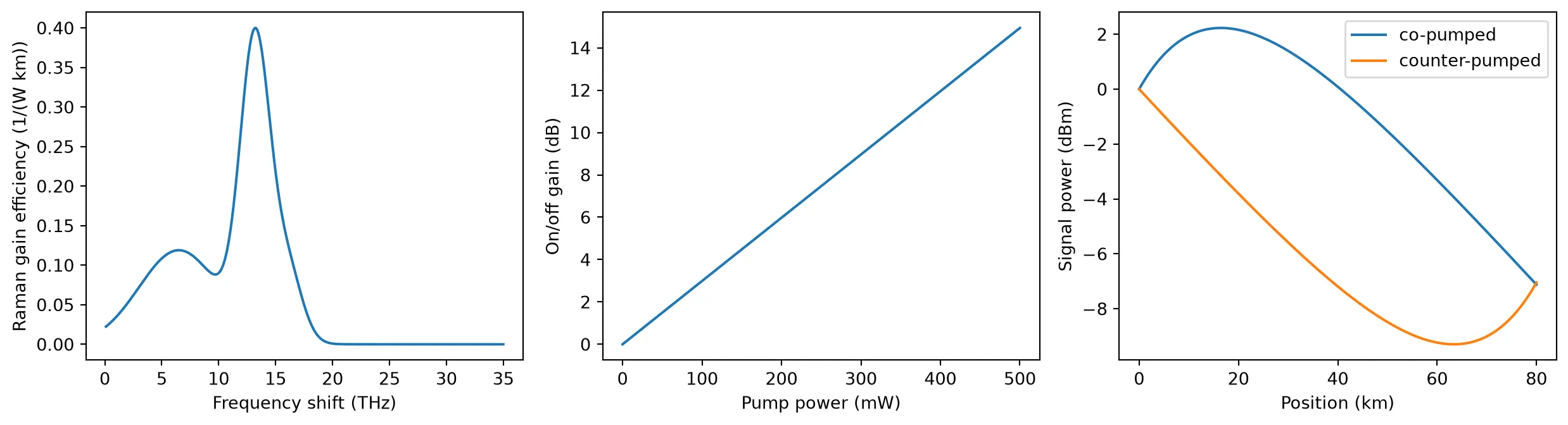

The Raman gain efficiency peaks at a shift of 13.2 THz, which places a 1450 nm pump’s gain at 1550 nm. The on/off gain grows linearly in dB with pump power, reaching about 9 dB at 300 mW over 80 km. The power profiles show that both pumping directions give nearly the same on/off gain, but in different places: the co-pumped signal is amplified near the input, where it is strongest, and the counter-pumped signal near the end, where it is weakest. Counter-pumping is the common choice for a reason the profiles do not show: the pump and the signal travel in opposite directions, so fluctuations of the pump power average out along the fiber instead of being copied onto the signal [2]. With a 1 mW signal the pump loses 3.3% of its power when co-pumped and 1.1% when counter-pumped, so the undepleted closed form and the coupled equations agree within 0.1 dB.

lengths_sbs = np.linspace(1, 100, 100)  # Fiber lengths (km)
linewidths = [0.0, 1e9, 10e9]  # Source linewidths (Hz)

fig, ax = plt.subplots(figsize=(6.5, 3.6), tight_layout=True)
for linewidth in linewidths:
    # Brillouin threshold against fiber length for this source linewidth (W)
    threshold = [
        pf.fiber.brillouin_threshold(length, source_linewidth=linewidth)
        for length in lengths_sbs
    ]

    # Legend label of this linewidth
    label = (
        "single frequency" if linewidth == 0 else f"{linewidth / 1e9:.0f} GHz linewidth"
    )
    ax.semilogy(lengths_sbs, np.array(threshold) * 1e3, label=label)
ax.set(xlabel="Fiber length (km)", ylabel="Brillouin threshold (mW)")
ax.legend()
plt.show()

for linewidth in linewidths:
    # Brillouin threshold of a 50 km fiber for this linewidth (W)
    p_th = pf.fiber.brillouin_threshold(50.0, source_linewidth=linewidth)
    print(f"50 km, {linewidth / 1e9:4.0f} GHz linewidth: threshold {p_th * 1e3:.1f} mW")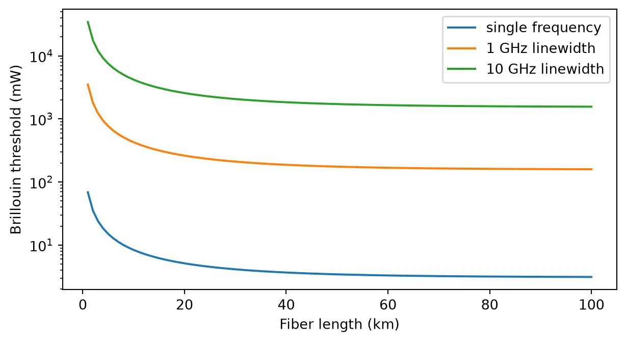

50 km,    0 GHz linewidth: threshold 3.4 mW
50 km,    1 GHz linewidth: threshold 175.4 mW
50 km,   10 GHz linewidth: threshold 1722.7 mW

A single-frequency source reaches the Brillouin threshold at only a few milliwatts in a 50 km fiber, 3.4 mW here. The threshold stops falling beyond a few tens of kilometers, because the effective length saturates at about $1/\alpha \approx 22$ km. Modulation broadens the spectrum: with a 10 GHz linewidth the threshold rises by a factor of about 500, to 1.7 W. Brillouin scattering therefore limits unmodulated carriers, such as the local oscillator or a remote laser source, and rarely limits modulated data channels.

Summary

• pfa.fiber models loss, chromatic dispersion and its slope, and the Kerr effect, from datasheet values. Its time stepper works in the frame that moves with the signal, so the output appears after the filter latency rather than the transit time.
• The Kerr effect is treated with the split-step method. peak_power sets the number of sections automatically, so that the nonlinear phase per section stays below max_phase; a linear fiber is a single section.
• pfa.pmd_fiber models polarization-mode dispersion with a Jones matrix. Each seed is one fiber, and the DGD over many fibers follows the Maxwellian distribution with mean $D_\mathrm{PMD}\sqrt{L}$. The time stepper applies the same Jones matrix, so a pulse split between the principal states arrives as two copies separated by the DGD.
• With dual_polarization=True, pfa.fiber carries both polarizations and connects directly to pmd_fiber to form a dual-polarization span, with the Manakov factor of 8/9 on the Kerr effect.
• The frequency-domain S matrix and the time stepper of each component describe the same fiber, so the S matrix of a span can be used to design or check the receiver processing.
• pf.fiber provides the unit conversions, the section and filter sizes, the Raman gain with co- and counter-pumping, and the Brillouin threshold.

References

1. G. P. Agrawal, Nonlinear Fiber Optics, 5th ed. (Academic Press, 2013).
2. G. P. Agrawal, Fiber-Optic Communication Systems, 4th ed. (Wiley, 2010).
3. J. P. Gordon and H. Kogelnik, “PMD fundamentals: Polarization mode dispersion in optical fibers,” Proc. Natl. Acad. Sci. USA 97, 4541 (2000).
4. D. Marcuse, C. R. Menyuk, and P. K. A. Wai, “Application of the Manakov-PMD equation to studies of signal propagation in optical fibers with randomly varying birefringence,” J. Lightwave Technol. 15, 1735 (1997).
5. S. J. Savory, “Digital coherent optical receivers: algorithms and subsystems,” IEEE J. Sel. Top. Quantum Electron. 16, 1164 (2010).
6. R. G. Smith, “Optical power handling capacity of low loss optical fibers as determined by stimulated Raman and Brillouin scattering,” Appl. Opt. 11, 2489 (1972).