LiDAR Grating Antenna Design

Download notebook (.zip)

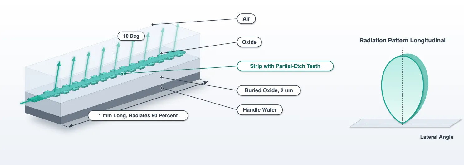
The technology page fixed the platform: 220 nm silicon on a 2 um buried oxide, a full etch and a partial etch that leaves a 70 nm slab, oxide up to 3.6 um and air above. It also fixed what the antenna has to do: radiate the light of a 500 nm strip over about a millimetre, 10 degrees off the surface normal, from 32 antennas 1.3 um apart. This page designs that antenna. Every number in it is measured here, and every later page uses them.

The design goes in six steps, each with one quantity to measure and one decision to take:

Pitch, from the field of view and the grating lobe. Geometry, no simulation.
Strip widths, from the coupling between neighbouring antennas. Mode solver.
Radiation strength, from the tooth duty cycle. Short FDTD runs in oxide alone.
Emission angle, from the radiation pattern in the real stack. FDTD with wafer and air.
The two antennas side by side: crosstalk and the pattern of each inside a row. FDTD.
From the simulated section to the real antenna. Arithmetic.

Two terms are used throughout. The radiation pattern, or element pattern, is the radiated power per unit solid angle in the air, per unit of power fed into the antenna, as a function of direction. The array factor is the interference of the 32 antennas’ fields, which the steering page multiplies into the pattern to get the beam.

# The technology, the wavelength grid, the strip index and the system numbers
from runpy import run_path

# Lidar_Technology.qmd defines what this notebook builds on. Its shared cells are
# generated into the module below; see docs/scripts/generate_notebook_modules.py.
globals().update(
    {k: v for k, v in run_path("misc/lidar_technology.py").items() if not k.startswith("_")}
)

from photonforge.live_viewer import LiveViewer

# Layout viewer for the cells built below
viewer = LiveViewer()

# Index of the design frequency in the shared wavelength grid, and the routing strip width
i0 = int(np.argmin(np.abs(freqs - f0)))
w_core = tech.parametric_kwargs["core_width"]

# Heights of the two interfaces that bound the stack, from the technology's own parameters
stack = tech.parametric_kwargs
z_wafer = -stack["box_thickness"]  # top of the handle wafer (um)
# oxide-air surface (um)
z_top = (
    stack["core_thickness"]
    + stack["heater_separation"]
    + stack["heater_thickness"]
    + stack["metal_separation"]
    + stack["metal_thickness"]
)
n_oxide = 1.444  # cladding index at 1550 nm

# Direction cosines for the k-space projection: kx/k0 longitudinal, ky/k0 lateral
u_grid = np.linspace(-1, 1, 161)

LiveViewer started at http://127.0.0.1:38077. Call its 'stop()' method to free the port.

Step 1: pitch

An array of antennas at pitch $d$ , fed with a linear phase ramp, radiates its beam at $\theta_0$ and its grating lobes at $\sin\theta = \sin\theta_0 \pm \lambda/d$ . A grating lobe inside the visible half-space is a second beam the LiDAR transmits into and receives from. The field of view is the steering range before the first grating lobe enters on the opposite side, $2\arcsin(\lambda/2d)$ .

For $d$ below the wavelength, $\lambda/d > 1$ and a broadside beam has no grating lobe in the visible half-space at all; the lobe enters only as the beam steers, at the far edge, where the radiation pattern of a narrow antenna is weak. At the 2 um pitch of Poulton et al. [1], the lobe of a broadside beam sits at 51 degrees, and their paper reports it as strong as the beam. The 1.3 um pitch of Zhang et al. [2] and Miller et al. [3] gives a 73 degree field of view and no lobe at broadside, and it is the pitch here. How far the lobe stays below the beam across the scan depends on the radiation pattern, so that check comes in step 4.

References

Poulton, C. V., et al. “Coherent solid-state LIDAR with silicon photonic optical phased arrays.” Optics Letters 2017 42 (20), 4091-4094, doi: 10.1364/OL.42.004091.
Zhang, Y., et al. “Sub-wavelength-pitch silicon-photonic optical phased array for large field-of-regard coherent optical beam steering.” Optics Express 2019 27 (3), 1929-1940, doi: 10.1364/OE.27.001929.
Miller, S. A., et al. “Large-scale optical phased array using a low-power multi-pass silicon photonic platform.” Optica 2020 7 (1), 3-6, doi: 10.1364/OPTICA.7.000003.
Ginel-Moreno, P., et al. “Millimeter-long metamaterial surface-emitting antenna in the silicon photonics platform.” Optics Letters 2021 46 (15), 3733-3736, doi: 10.1364/OL.431983.
Raval, M., et al. “Unidirectional waveguide grating antennas with uniform emission for optical phased arrays.” Optics Letters 2017 42 (13), 2563-2566, doi: 10.1364/OL.42.002563.

print("pitch   field of view   grating lobe of a broadside beam")
for d in (2.0, 1.6, 1.3):
    u_lobe = lda0 / d
    lobe = (
        f"{np.degrees(np.arcsin(u_lobe)):.0f} deg"
        if u_lobe < 1
        else "none in the visible half-space"
    )
    print(
        f"{d:.1f} um    {2 * np.degrees(np.arcsin(lda0 / (2 * d))):5.1f} deg       {lobe}"
    )
print(f"\nchosen: {pitch} um, the value the system budget carries")

pitch   field of view   grating lobe of a broadside beam
2.0 um     45.6 deg       51 deg
1.6 um     57.9 deg       76 deg
1.3 um     73.2 deg       none in the visible half-space

chosen: 1.3 um, the value the system budget carries

Step 2: strip widths

At 1.3 um pitch two 500 nm strips are 0.8 um apart. Two identical waveguides that close exchange their light completely over the coupling length $L_c = \lambda / (2\,\Delta n)$ , where $\Delta n$ is the index difference of the even and odd modes of the pair. If $L_c$ is comparable to the antenna length, the array is not 32 antennas but one wide slab of them.

Detuning removes the coupling. Two waveguides of different width have different propagation constants $\beta_1$ and $\beta_2$ , and coupled-mode theory bounds the power that can ever cross between them:

F_\text{max} = \frac{\kappa^2}{\kappa^2 + (\Delta\beta / 2)^2}, \qquad \kappa = \frac{\pi \Delta n}{\lambda}, \qquad \Delta\beta = \beta_1 - \beta_2 .

The mode solver gives every number in that expression. The cell below solves the even and odd modes of two 500 nm strips at the pitch, and the mode of a 450 nm strip, which is still a comfortable single-mode width. Alternating the two widths down the array gives every antenna a detuned neighbour on both sides. The cost is a second antenna design: the narrower strip needs its own period and duty cycle, worked out alongside the first in the steps that follow.

def strip_spec(width, offsets=(0.0,), num_modes=1):
    """Port specification for one or more strips of the given width at the given lateral offsets."""
    return pf.PortSpec(
        description=f"{len(offsets)} strip(s) of {width * 1e3:.0f} nm",
        width=max(offsets)
        - min(offsets)
        + 3.0,  # simulation window, wide enough for the tails
        limits=(-1.0, 1.0),
        num_modes=num_modes,
        target_neff=3.5,  # the core index, a search hint for the mode solver
        path_profiles=[(width, y, (1, 0)) for y in offsets],
    )

width_second = 0.45  # The alternate strip width (um)
l_budget = 1050.0  # The antenna length the technology page's budget carries (um)

# Even and odd modes of two identical strips at the pitch, and the single strips' own indices
pair = pf.port_modes(
    strip_spec(w_core, (-pitch / 2, pitch / 2), num_modes=2),
    [f0],
    show_progress=False,
    verbose=False,
)
n_pair = np.sort(np.real(pair.data.n_eff.values.ravel()))[::-1]
second = pf.port_modes(
    strip_spec(width_second), [f0], show_progress=False, verbose=False
)
n_second = float(np.real(second.data.n_eff.values.ravel()[0]))

# Coupling of the identical pair, and the bound with the detuning of the second width
kappa = np.pi * (n_pair[0] - n_pair[1]) / lda0
l_coupling = np.pi / (2 * kappa)
delta_beta = 2 * np.pi / lda0 * (n_eff_strip - n_second)
f_max = kappa**2 / (kappa**2 + (delta_beta / 2) ** 2)
print(
    f"two 500 nm strips at {pitch} um pitch: even and odd modes {n_pair[0]:.4f} and {n_pair[1]:.4f}, "
    f"coupling length {l_coupling:.0f} um; over {l_budget:.0f} um the light would cross "
    f"{np.sin(kappa * l_budget) ** 2 * 100:.0f} percent"
)
print(
    f"{width_second * 1e3:.0f} nm strip: n_eff {n_second:.4f}, {n_eff_strip - n_second:.4f} below the 500 nm strip; "
    f"at most {f_max * 100:.2f} percent ({10 * np.log10(f_max):.0f} dB) ever crosses between the two"
)

two 500 nm strips at 1.3 um pitch: even and odd modes 2.4392 and 2.4390, coupling length 6046 um; over 1050 um the light would cross 7 percent
450 nm strip: n_eff 2.3475, 0.0916 below the 500 nm strip; at most 0.00 percent (-57 dB) ever crosses between the two

Step 3: radiation strength

A grating antenna is a waveguide with a periodic perturbation weak enough that the guided mode leaks into one radiating order over a long distance. The guided power falls as

P(x) = P_0\, e^{-2 \alpha x},

and the antenna has to be long enough to empty the waveguide: radiating 90 percent takes $L_{90} = \ln 10 / (2\alpha)$ . The budget carries an antenna of about a millimetre, so the target is 10 dB per millimetre, which is a weak grating. A perturbation on top of the waveguide, where the mode is strongest, radiates far too fast at any depth the fabrication holds [4]. The perturbation here is on the sidewalls, as in Poulton’s chip [1], but in the partial etch: each tooth is a 70 nm tall shoulder beside the full-height strip.

The tooth has two dimensions. Its width, how far it sticks out across the antenna, is fixed at 100 nm, the smallest feature the partial etch is allowed, so that the design does not depend on the fabrication holding anything finer. Its duty cycle, the fraction of each period it occupies along the antenna, is the design knob: a corrugation with duty cycle $D$ has a first Fourier coefficient proportional to $\sin(\pi D)$ , so the strength is largest at 50 percent and falls as the tooth shortens. The sweep below measures the strength at 50 and 25 percent for both widths and fits a power law through the two points. The duty cycle for 10 dB/mm follows from the law and a third run confirms it. If the confirmation misses by more than 0.5 dB/mm, the two nearest points give a corrected law and one more run. The tooth’s extent along the antenna is rounded to the 5 nm grid of the mask.

Two simplifications keep these runs under one FlexCredit each. First, the decay rate is a property of the guided mode, so the wafer and the air above the cladding are left out. The runs are in oxide alone, in a window 3 um wide and 2.6 um tall; step 4 confirms that the stack changes the rate by well under a percent. Second, twenty periods, about 15 um, are enough: a few percent of the light leaves the waveguide, and the S matrix resolves that to a fraction of a percent. The mesh is refined to 20 nm along and across the teeth, since the tooth’s extent along the antenna is the quantity being varied. Each run also carries a k-space projection monitor above the grating. Its peak gives the emission angle and, through the grating equation, the index the teeth add to the strip; step 4 needs both.

@pf.parametric_component(name_prefix="ANT")
def grating_antenna(
    *,
    period=0.74,
    tooth=0.10,
    duty=0.25,
    width=0.5,
    num_periods=20,
    lead=1.0,
    taper=2.0,
    overlap=0.0
):
    # Empty name, so the decorator builds one from the arguments
    c = pf.Component()
    port_spec = pf.config.default_technology.ports["TE_1550_500"]
    l_grating = num_periods * period
    # the helpers below read the grating length from here
    c.properties["l_grating"] = l_grating

    # A strip narrower than the routing waveguide gets a linear taper at each end
    l_taper = 0.0 if abs(width - w_core) < 1e-9 else taper
    c.add("Si", pf.Rectangle((-(lead + l_taper), -w_core / 2), (-l_taper, w_core / 2)))
    c.add(
        "Si",
        pf.Rectangle(
            (l_grating + l_taper, -w_core / 2), (l_grating + lead + l_taper, w_core / 2)
        ),
    )
    # The exit taper may reach `overlap` into the grating, so that the two polygons' edges, snapped
    # to the mask grid separately, cannot leave a slit between them on a long antenna
    if l_taper > 0:
        c.add("Si", pf.Path((-l_taper, 0), w_core).segment((0, 0), width=width))
        c.add(
            "Si",
            pf.Path((l_grating - overlap, 0), width).segment(
                (l_grating + l_taper, 0), width=w_core
            ),
        )

    # The full-height strip through the grating
    c.add("Si", pf.Rectangle((0, -width / 2), (l_grating, width / 2)))

    # A partial-etch tooth on both sidewalls, its extent along the antenna on the 5 nm mask grid
    l_tooth = round(duty * period / 0.005) * 0.005
    for i in range(num_periods):
        x_tooth = i * period
        c.add(
            "Si Partial",
            pf.Rectangle(
                (x_tooth, -width / 2 - tooth), (x_tooth + l_tooth, width / 2 + tooth)
            ),
        )

    # Both leads end in the plain routing strip, so the ports are found from the geometry
    c.add_port(c.detect_ports([port_spec]))

    # Standard grid everywhere, 20 nm cells along and across the toothed sidewalls only
    grid = td.GridSpec.auto(
        wavelength=lda0,
        min_steps_per_wvl=14,
        override_structures=[
            td.MeshOverrideStructure(
                geometry=td.Box(
                    center=(l_grating / 2, sign * (width + tooth) / 2, 0.11),
                    size=(l_grating, tooth + 0.2, 0.3),
                ),
                dl=(0.02, 0.02, None),
            )
            for sign in (-1, 1)
        ],
    )

    # In oxide alone: a z window of +-1.3 um leaves the wafer and the air outside. The k-space
    # monitor in the oxide gives the emission direction, in the oxide's own direction cosines.
    monitors = [
        td.FieldProjectionKSpaceMonitor(
            center=(l_grating / 2, 0, 1.0),
            size=(td.inf, td.inf, 0),
            freqs=freqs,
            name="far",
            normal_dir="+",
            proj_axis=2,
            proj_distance=1e6,
            ux=u_grid,
            uy=u_grid,
        )
    ]
    c.add_model(
        pf.Tidy3DModel(
            monitors=monitors,
            grid_spec=grid,
            bounds=((None, None, -1.3), (None, None, 1.3)),
            verbose=False,
        ),
        "FDTD",
    )
    return c

# An arbitrary design, drawn to show the parts: leads, tapers, the strip and the teeth
viewer(grating_antenna(period=0.70, duty=0.5, width=0.45, num_periods=6))

Two helpers read a cell’s run. strength turns the transmission of the section into the decay rate and reads the emission angle off the k-space monitor; tooth_grid snaps a duty cycle to the mask grid. The sweep then submits its four runs together, fits the power law and confirms it.

def strength(cell):
    """Decay rate of one antenna cell: dB per millimetre, alpha in 1/um, the 90 percent length,
    and the emission angle in air at every wavelength, from its cached run."""
    s = cell.s_matrix(freqs, model_kwargs={"inputs": ["P0"]})
    transmitted = np.abs(s[("P0@0", "P1@0")]) ** 2
    l_grating = cell.properties["l_grating"]
    alpha = -np.log(transmitted[i0]) / (2 * l_grating)
    # Emission angle: the longitudinal cut of the k-space monitor peaks at kx = n_ox k0 ux; in air sin(theta) = n_ox ux
    data = next(
        iter(cell.models["FDTD"].batch_data(cell, freqs, inputs=["P0"]).values())
    )
    far = data["far"].power.isel(r=0).transpose("ux", "uy", "f").values
    longitudinal = far[:, np.argmin(np.abs(u_grid)), :]
    angles = np.degrees(
        np.arcsin(np.clip(n_oxide * u_grid[np.argmax(longitudinal, axis=0)], -1, 1))
    )
    return dict(
        transmitted=transmitted,
        alpha=alpha,
        db_per_mm=-10 * np.log10(transmitted[i0]) / (l_grating * 1e-3),
        l90=np.log(10) / (2 * alpha),
        angle=float(angles[i0]),
        angles=angles,
        longitudinal=longitudinal,
    )

def tooth_grid(duty, period):
    """The duty cycle whose tooth extent along the antenna lies on the 5 nm mask grid."""
    return round(duty * period / 0.005) * 0.005 / period

target_db_per_mm = 10.0  # radiates 90 percent in one millimetre
tolerance_db_per_mm = 0.5
tooth = 0.10  # tooth width across the antenna: the partial etch's smallest feature (um)

# Starting periods from the plain strips' indices and the design angle; the teeth add index, so
# the measured emission angle corrects them at the confirmation
strips = {w_core: n_eff_strip, width_second: n_second}
design = {
    w: dict(period=lda0 / (n - np.sin(np.radians(theta0)))) for w, n in strips.items()
}

# The two sweep points for each width, all four submitted before any is read
duties = (0.5, 0.25)
runs = {
    w: {
        D: grating_antenna(
            period=d["period"], tooth=tooth, duty=tooth_grid(D, d["period"]), width=w
        )
        for D in duties
    }
    for w, d in design.items()
}
for cells_of_width in runs.values():
    for cell in cells_of_width.values():
        cell.models["FDTD"].start(cell, freqs, inputs=["P0"])
print("four sweep runs submitted")

four sweep runs submitted

The runs come back and the power law is fitted through the two points of each width.

results = {
    w: {D: strength(cell) for D, cell in cells_of_width.items()}
    for w, cells_of_width in runs.items()
}

for w, d in design.items():
    # Power law through the two points, and the duty cycle it predicts for the target
    D1, D2 = duties
    s1, s2 = results[w][D1]["db_per_mm"], results[w][D2]["db_per_mm"]
    exponent = np.log(s1 / s2) / np.log(D1 / D2)
    d["duty"] = tooth_grid(D2 * (target_db_per_mm / s2) ** (1 / exponent), d["period"])
    # The grating index each run implies, and its slope with duty, correct the period
    n_avg = {
        D: np.sin(np.radians(results[w][D]["angle"])) + lda0 / d["period"]
        for D in duties
    }
    d["n_avg_slope"] = (n_avg[D1] - n_avg[D2]) / (D1 - D2)
    d["n_avg"] = n_avg[D2] + d["n_avg_slope"] * (d["duty"] - D2)
    d["period"] = lda0 / (d["n_avg"] - np.sin(np.radians(theta0)))
    d["history"] = [(D, results[w][D]["db_per_mm"]) for D in duties]
    d["exponent"] = exponent

A confirmation run at the predicted duty cycle for each width, both submitted together, and one correction if either misses the tolerance.

# Confirmation runs, both widths together; a second correction if either misses the tolerance
for attempt in range(2):
    cells = {
        w: grating_antenna(period=d["period"], tooth=tooth, duty=d["duty"], width=w)
        for w, d in design.items()
    }
    for cell in cells.values():
        cell.models["FDTD"].start(cell, freqs, inputs=["P0"])
    for w, d in design.items():
        r = strength(cells[w])
        d["history"].append((d["duty"], r["db_per_mm"]))
        d["cell"], d["result"] = cells[w], r
        print(
            f"attempt {attempt + 1}, {w * 1e3:.0f} nm strip at {d['duty'] * 100:.1f} percent: {r['db_per_mm']:.1f} dB/mm"
        )
    if all(
        abs(d["result"]["db_per_mm"] - target_db_per_mm) <= tolerance_db_per_mm
        for d in design.values()
    ):
        break
    for w, d in design.items():
        if abs(d["result"]["db_per_mm"] - target_db_per_mm) > tolerance_db_per_mm:
            # The two nearest points give the local law; the angle just measured gives the index
            (D1, s1), (D2, s2) = d["history"][-2], d["history"][-1]
            d["exponent"] = np.log(s1 / s2) / np.log(D1 / D2)
            d["duty"] = tooth_grid(
                D2 * (target_db_per_mm / s2) ** (1 / d["exponent"]), d["period"]
            )
        d["n_avg"] = np.sin(np.radians(d["result"]["angle"])) + lda0 / d["period"]
        d["period"] = lda0 / (d["n_avg"] - np.sin(np.radians(theta0)))

attempt 1, 500 nm strip at 27.8 percent: 10.2 dB/mm
attempt 1, 450 nm strip at 18.9 percent: 8.1 dB/mm
attempt 2, 500 nm strip at 27.8 percent: 10.3 dB/mm
attempt 2, 450 nm strip at 21.2 percent: 9.7 dB/mm

The sweep points, the law and the confirmation in one table, and the antenna length that follows from the decay rates.

print("width   duty    tooth length  period   T        dB/mm   L90 (um)   emission")
for w, d in design.items():
    for D, s in d["history"][:-1]:
        print(
            f"{w * 1e3:3.0f} nm  {D * 100:5.1f} %   sweep                                {s:5.1f}"
        )
    r = d["result"]
    print(
        f"{w * 1e3:3.0f} nm  {d['duty'] * 100:5.1f} %   {d['duty'] * d['period'] * 1e3:5.0f} nm      {d['period'] * 1e3:3.0f} nm   "
        f"{r['transmitted'][i0]:.4f}   {r['db_per_mm']:5.1f}   {r['l90']:7.0f}    {r['angle']:5.1f} deg   <- chosen"
    )
    print(
        f"        strength falls as duty cycle to the power {d['exponent']:.1f}; grating index {d['n_avg']:.4f} "
        f"against {strips[w]:.4f} for the plain strip"
    )

# Antenna length for the series: the longer of the two 90 percent lengths, rounded to 50 um
l_antenna = 50 * round(max(d["result"]["l90"] for d in design.values()) / 50)
print(
    f"\nantenna length {l_antenna:.0f} um (the budget carries {l_budget:.0f} um); the antennas radiate "
    + " and ".join(
        f"{(1 - np.exp(-2 * d['result']['alpha'] * l_antenna)) * 100:.0f} percent"
        for d in design.values()
    )
    + " of their light over it"
)

width   duty    tooth length  period   T        dB/mm   L90 (um)   emission
500 nm   50.0 %   sweep                                 18.8
500 nm   25.0 %   sweep                                  8.9
500 nm   27.8 %   sweep                                 10.2
500 nm   27.8 %     189 nm      679 nm   0.9682    10.3       968     10.4 deg   <- chosen
        strength falls as duty cycle to the power 1.1; grating index 2.4548 against 2.4391 for the plain strip
450 nm   50.0 %   sweep                                 24.4
450 nm   25.0 %   sweep                                 12.8
450 nm   18.9 %   sweep                                  8.1
450 nm   21.2 %     151 nm      710 nm   0.9686     9.7      1026     10.4 deg   <- chosen
        strength falls as duty cycle to the power 1.6; grating index 2.3568 against 2.3475 for the plain strip

antenna length 1050 um (the budget carries 1050 um); the antennas radiate 92 percent and 91 percent of their light over it

fig, ax = plt.subplots(1, 1, figsize=(6, 4))
for w, d in design.items():
    D_pts, s_pts = zip(*d["history"])
    (line,) = ax.loglog(
        np.array(D_pts) * 100, s_pts, "o", label=f"{w * 1e3:.0f} nm strip, simulated"
    )
    D_fit = np.linspace(0.1, 0.5, 50)
    ax.loglog(
        D_fit * 100,
        s_pts[-1] * (D_fit / D_pts[-1]) ** d["exponent"],
        "--",
        color=line.get_color(),
        linewidth=0.8,
    )
ax.axhline(target_db_per_mm, color="gray", linestyle=":", linewidth=1)
ax.set_xlabel("duty cycle (%)")
ax.set_ylabel("radiation strength (dB/mm)")
ax.legend()
plt.show()

# The 500 nm antenna's numbers under the names the later pages read
period_chosen, duty_chosen, tooth_chosen = (
    design[w_core]["period"],
    design[w_core]["duty"],
    tooth,
)
n_avg_chosen, antenna = design[w_core]["n_avg"], design[w_core]["result"]
duty_exponent = design[w_core]["exponent"]
l_tooth_chosen = duty_chosen * period_chosen
antenna_cell, second_cell = design[w_core]["cell"], design[width_second]["cell"]
l_section = antenna_cell.properties["l_grating"]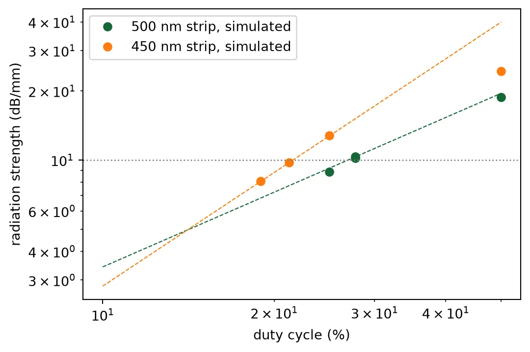

Three results follow from the table.

A 100 nm partial-etch shoulder is a strong perturbation. At 50 percent duty cycle it radiates twice what a millimetre antenna needs, so the duty cycle, not the width, is the design variable. The strength falls as a power of the duty cycle between 1 and 1.5, close to the $\sin^2(\pi D)$ of a thin corrugation; a short tooth also perturbs the mode less per unit length.
The narrower strip radiates more with the same teeth, since its mode is less confined and reaches the shoulders more. It therefore ends up with a shorter tooth.
The teeth add index. The emission angle of the sweep cells lies above the angle the period was cut for, by an amount that grows with the duty cycle. The confirmation runs at the corrected period emit within a fraction of a degree of the design angle.

Both antennas now radiate at the target rate, and the antenna length follows from it.

Step 4: emission angle and the radiation pattern

The stack decides where the radiated light goes as much as the grating does. A sidewall grating radiates downward as well as upward. Two micrometres below the core the oxide meets the silicon wafer, whose reflectivity for light arriving from the oxide is 17 percent. The reflected light comes back up through the core and interferes with the light that went up directly, with a phase that depends on the direction. The radiation pattern in the air therefore has bright and dark directions that the grating alone would not have. Raval et al. [5] measured such fringes and showed that they cost several decibels at the dark angles. Which directions are bright depends on the buried-oxide thickness, which the foundry fixes, and on the emission angle, which the period sets. The emission angle is therefore chosen by measuring the pattern in the real stack at candidate angles.

The measurement is a run of the chosen 500 nm antenna with the wafer below and the air above. The window is 20 um wide in the lateral direction, because light reflected by the wafer travels sideways for several micrometres before it reaches the surface, and a narrow window would cut it off. The k-space projection monitor sits in the air a quarter micrometre above the surface. It returns the radiated power per unit solid angle in the air against the two direction cosines, $k_x/k_0$ along the antenna (longitudinal) and $k_y/k_0$ across it (lateral). Two flux planes, one in the air and one in the wafer, split the radiated power into what leaves the chip and what is lost below. Each run bills about one FlexCredit. The candidate angles are the 10 degrees the technology page set and 20 degrees, a tilt that gratings on thinner buried oxides often use; both runs are submitted together.

Three views of the result are drawn: the map of radiated power against direction, its longitudinal cut at $k_y = 0$ , and its lateral cut through the emission peak. Directions are given by the two angles the phased-array literature uses (Hulme et al., Opt. Express 23, 5861 (2015)): the longitudinal angle $\theta$ , measured from the surface normal in the plane that contains the antenna, which the grating period sets and the wavelength steers, and the lateral angle $\psi$ , measured from the normal in the plane perpendicular to the antenna, which the phases steer; $\sin\psi = k_y/k_0$ . The lateral cut is the pattern against $\psi$ through the emission peak, and it is the radiation pattern the array factor multiplies. It has to be taken through the peak. At $k_x = 0$ , the plane through the surface normal where far fields are usually drawn, the longitudinal cut of a short section is some 40 dB down, and whatever weak light exists there dominates.

As simulated, the two test sections differ. Both have 20 periods, and a larger angle means a longer period, so the 20 degree section is 8 percent longer. At the same duty cycle its teeth are longer too, so it radiates more power over its length. Neither difference exists in the finished antennas, which are both a millimetre long and radiate 90 percent of their light. Two normalizations remove them. The pattern is divided by the power the section radiated and by the section length. The second normalization is needed because the longitudinal lobe of a section is $\lambda/L$ wide: at the same radiated power a longer section puts its light into a narrower lobe, and its peak per steradian is taller in proportion to $L$ . What remains is the intensity that a millimetre-long antenna would give per unit of radiated power. It is compared at three points read from each pattern:

share reaching the air: the power through the flux plane in the air divided by the power the section radiated;
weakest beam in the scan: the smallest value of the pattern over the lateral-steering range the array will use, ±20 degrees, since a beam steered there carries that much;
grating-lobe level: over that same range, the largest ratio of the pattern at the grating lobe’s direction to the pattern at the beam’s direction, in dB, for the 1.3 um pitch.

The measured intensity already contains the loss of projected aperture at a tilted emission, the factor $\cos\theta_0$ by which the beam widens longitudinally, so nothing is added for it.

half_width = 10.0  # Half the lateral width of the window (um)

def radiation_monitors(l_grating, frequencies):
    """Flux planes a quarter micrometre into the air and into the wafer, and the k-space projection
    on the air plane, whose direction cosines are those of the light leaving the chip.
    """
    z_air, z_si = z_top + 0.25, z_wafer - 0.25
    return [
        td.FluxMonitor(
            center=(l_grating / 2, 0, z_air),
            size=(td.inf, td.inf, 0),
            freqs=frequencies,
            name="up",
        ),
        td.FluxMonitor(
            center=(l_grating / 2, 0, z_si),
            size=(td.inf, td.inf, 0),
            freqs=frequencies,
            name="down",
        ),
        td.FieldProjectionKSpaceMonitor(
            center=(l_grating / 2, 0, z_air),
            size=(td.inf, td.inf, 0),
            freqs=frequencies,
            name="far",
            normal_dir="+",
            proj_axis=2,
            proj_distance=1e6,
            ux=u_grid,
            uy=u_grid,
        ),
    ]

def antenna_row(row_cells, name):
    """The given antenna cells side by side at the array pitch, in the real stack and the wide
    window, on the standard mesh, at the design wavelength. Every lead is a port whose mode
    window holds one strip only: the standard 3 um window reaches into the neighbours at the
    1.3 um pitch, and a strip cut by the edge of the window carries a spurious mode of higher
    index that the mode solver would launch instead of the strip's own."""
    c = pf.Component(name)
    row_spec = pf.config.default_technology.ports["TE_1550_500"].copy()
    # one strip and its evanescent tail, no neighbour inside the window
    row_spec.width = 2.0
    ys = (np.arange(len(row_cells)) - (len(row_cells) - 1) / 2) * pitch
    for k, (cell, y) in enumerate(zip(row_cells, ys)):
        ref = c.add_reference(cell).translate((0, y))
        c.add_port(
            pf.Port(ref["P0"].center, ref["P0"].input_direction, row_spec), f"IN{k}"
        )
        c.add_port(
            pf.Port(ref["P1"].center, ref["P1"].input_direction, row_spec), f"OUT{k}"
        )
    c.add_model(
        pf.Tidy3DModel(
            monitors=radiation_monitors(l_section, [f0]),
            grid_spec=12,
            verbose=False,
            bounds=(
                (None, -half_width, z_wafer - 0.4),
                (None, half_width, z_top + 1.0),
            ),
        ),
        "FDTD",
    )
    c.properties["l_grating"] = l_section
    return c

def radiation(cell, port_in, port_out):
    """Transmitted fraction, radiated fraction, and the shares of the radiated light that reach the
    air, enter the wafer, or stay trapped in the cladding, from a stack run at the design wavelength.
    """
    s = cell.s_matrix([f0], model_kwargs={"inputs": [port_in]})
    transmitted = abs(s[(f"{port_in}@0", f"{port_out}@0")][0]) ** 2
    data = next(
        iter(cell.models["FDTD"].batch_data(cell, [f0], inputs=[port_in]).values())
    )
    up, down = float(data["up"].flux.values[0]), -float(data["down"].flux.values[0])
    radiated = 1 - transmitted
    return dict(
        transmitted=transmitted,
        radiated=radiated,
        to_air=up / radiated,
        to_wafer=down / radiated,
        trapped=1 - (up + down) / radiated,
    )

def spectrum(cell, port="P0", frequencies=None):
    """Radiated power per unit solid angle against (kx/k0, ky/k0), one map per wavelength."""
    frequencies = freqs if frequencies is None else frequencies
    data = next(
        iter(cell.models["FDTD"].batch_data(cell, frequencies, inputs=[port]).values())
    )
    far = data["far"].power.isel(r=0).transpose("ux", "uy", "f")
    return far.ux.values, far.uy.values, far.values

def cuts(ux, uy, power, i_lda=0):
    """Longitudinal cut at ky = 0, its peak index per wavelength, and the lateral cut through the
    peak at one wavelength against the lateral angle in air."""
    longitudinal = power[:, np.argmin(np.abs(uy)), :]
    i_peak = np.argmax(longitudinal, axis=0)
    # directions on the cut that leave the chip
    inside = ux[i_peak[i_lda]] ** 2 + uy**2 < 1
    return (
        longitudinal,
        i_peak,
        np.degrees(np.arcsin(uy[inside])),
        power[i_peak[i_lda], inside, i_lda],
    )

def plot_spectrum(spectra, title):
    """The three views of one or more spectra on one absolute scale: the map, the longitudinal cut
    and the lateral cut through the peak. spectra maps a label to (ux, uy, power at one wavelength).
    """
    n = len(spectra)
    fig = plt.figure(figsize=(15, 3.8 * n))
    gs = fig.add_gridspec(n, 3, width_ratios=[1.1, 1, 1])
    ref = max(power.max() for _, _, power in spectra.values())
    ax_long, ax_lat = fig.add_subplot(gs[:, 1]), fig.add_subplot(gs[:, 2])
    for row, (label, (ux, uy, power)) in enumerate(spectra.items()):
        ax = fig.add_subplot(gs[row, 0])
        pcm = ax.pcolormesh(
            ux,
            uy,
            10 * np.log10(power.T / ref + 1e-9),
            vmin=-40,
            vmax=0,
            cmap="magma",
            shading="auto",
        )
        ax.set_aspect("equal")
        ax.set_xlabel("kx / k0, longitudinal")
        ax.set_ylabel("ky / k0, lateral")
        ax.set_title(f"{label}: radiated power (dB)")
        plt.colorbar(pcm, ax=ax, shrink=0.85)
        longitudinal, i_peak, theta_lateral, lateral = cuts(ux, uy, power[:, :, None])
        ax_long.semilogy(ux, longitudinal[:, 0] / ref, label=label)
        ax_lat.plot(theta_lateral, lateral / ref, label=label)
    ax_long.axvline(0, color="k", linewidth=0.6)
    ax_long.set_ylim(1e-4, 1.5)
    ax_long.set_xlabel("kx / k0")
    ax_long.set_title("longitudinal cut, ky = 0")
    ax_long.legend(fontsize=8)
    ax_lat.set_ylim(0, 1.3)
    ax_lat.set_xlabel("lateral angle, in air (deg)")
    ax_lat.set_title("lateral cut, through the peak")
    ax_lat.legend(fontsize=8)
    fig.suptitle(title)
    plt.tight_layout()
    plt.show()

# The 500 nm antenna at the two candidate angles, in the real stack, submitted together
alternative = 20.0  # The other candidate emission angle (deg)
candidates = {theta0: antenna_cell}
period_alt = lda0 / (n_avg_chosen - np.sin(np.radians(alternative)))
candidates[alternative] = grating_antenna(
    period=period_alt, tooth=tooth, duty=duty_chosen
)
patterns = {
    angle: antenna_row([cell], f"antenna_alone_{angle:.0f}deg")
    for angle, cell in candidates.items()
}
for row in patterns.values():
    row.models["FDTD"].start(row, [f0], inputs=["IN0"])

measured = {}
for angle, row in patterns.items():
    ux, uy, power = spectrum(row, port="IN0", frequencies=[f0])
    shares = radiation(row, "IN0", "OUT0")
    # Per unit radiated power and per unit section length: the footing a millimetre antenna gives
    power = power / (shares["radiated"] * candidates[angle].properties["l_grating"])
    longitudinal, i_peak, theta_lateral, lateral = cuts(ux, uy, power)
    measured[angle] = dict(
        ux=ux,
        uy=uy,
        power=power[:, :, 0],
        theta=theta_lateral,
        lateral=lateral,
        length=candidates[angle].properties["l_grating"],
        emission=float(np.degrees(np.arcsin(ux[i_peak[0]]))),
        **shares,
    )
plot_spectrum(
    {
        f"emission at {angle:.0f} deg": (m["ux"], m["uy"], m["power"])
        for angle, m in measured.items()
    },
    "the 500 nm antenna in the real stack, 1550 nm, per unit radiated power and section length",
)

def steering_metrics(theta_lateral, lateral, pitch_um, scan=20.0):
    """Weakest beam over a lateral steering range of +/-scan degrees and the worst grating-lobe
    level over it, from a radiation pattern against the lateral angle in air."""
    value = lambda u: np.interp(
        u, np.sin(np.radians(theta_lateral)), lateral, left=0.0, right=0.0
    )
    u_lobe = lda0 / pitch_um
    scan_u = np.sin(np.radians(np.arange(-scan, scan + 0.1, 2.0)))
    beam = np.array([value(u) for u in scan_u])
    lobes = np.array(
        [
            max(
                [value(u + s * u_lobe) for s in (-1, 1) if abs(u + s * u_lobe) < 1]
                or [0.0]
            )
            for u in scan_u
        ]
    )
    return beam.min(), 10 * np.log10(max(lobes / beam))

def half_width_deg(theta, pattern):
    """Full width at half maximum of a pattern against an angle in degrees."""
    above = theta[pattern > pattern.max() / 2]
    return above.max() - above.min()

scale = measured[theta0]["lateral"].max()
# lateral angle at the edge of the field of view
edge = np.degrees(np.arcsin(lda0 / (2 * pitch)))
print(
    "emission   simulated  section: length, radiated   share to air   lateral width  at broadside   "
    f"weakest over +/-20 deg   at the field edge ({edge:.0f} deg)   grating lobe"
)
for angle, m in measured.items():
    weakest, lobe = steering_metrics(m["theta"], m["lateral"], pitch)
    print(
        f"{angle:5.0f} deg   {m['emission']:5.1f} deg     {m['length']:5.1f} um, {m['radiated'] * 100:4.1f} %         "
        f"{m['to_air']:.2f}          {half_width_deg(m['theta'], m['lateral']):3.0f} deg         "
        f"{np.interp(0, m['theta'], m['lateral']) / scale:.2f}              {weakest / scale:.2f}                     "
        f"{np.interp(edge, m['theta'], m['lateral']) / scale:.2f}                    {lobe:+5.1f} dB"
    )
print(
    f"(pattern values per unit radiated power and section length, relative to the peak of the {theta0:.0f} deg pattern)"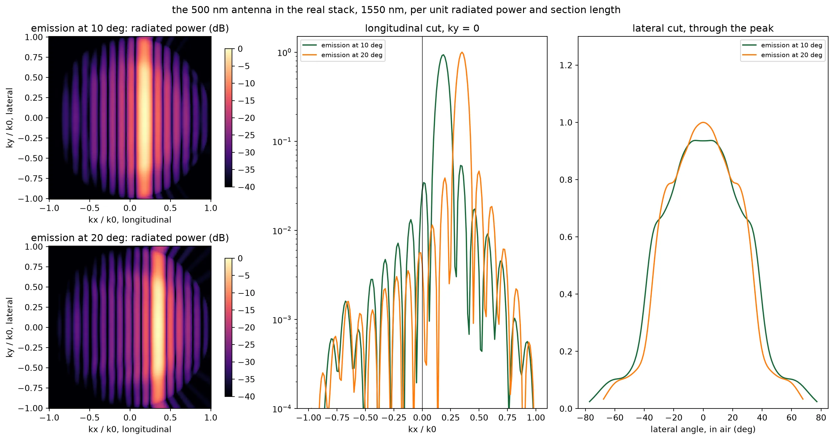
)

emission   simulated  section: length, radiated   share to air   lateral width  at broadside   weakest over +/-20 deg   at the field edge (37 deg)   grating lobe
   10 deg    10.8 deg      13.6 um,  3.3 %         0.48           76 deg         1.00              0.82                     0.57                     -8.7 dB
   20 deg    20.5 deg      14.7 um,  4.0 %         0.47           67 deg         1.07              0.85                     0.35                     -9.2 dB
(pattern values per unit radiated power and section length, relative to the peak of the 10 deg pattern)

Both patterns peak near normal, and both send half the radiated light into the air. The other half is lost into the wafer or trapped in the cladding by total internal reflection at the surface. On the equal footing the two are nearly the same pattern. The 20 degree one is a little narrower laterally, 67 degrees wide at half maximum against 76. At a larger tilt the polar angle, and with it the phase of the wafer reflection, changes faster with the lateral angle. The 20 degree pattern is a quarter of a decibel brighter at broadside and a tenth of a decibel brighter at the edge of the ±20 degree scan. Beyond 30 degrees it is weaker, and the 10 degree pattern holds up better toward the edge of the 73 degree field. The grating-lobe level is the same. The emission angle therefore does not change the radiated power, and the pattern needs to be measured once, not swept. The 10 degrees of the technology page are kept: the module looks close to the chip normal, and the pattern is the more even one over the field of view.

Step 5: the two antennas side by side

Step 2 bounded the coupling between the two widths from their modes. This step measures it, and it measures what the neighbours do to each antenna’s pattern. Two runs in the real stack and the wide window hold a row of three antennas at the pitch with the widths alternating and the middle one fed: once with the 500 nm antenna in the middle and once with the 450 nm antenna. The power that appears at the far ends of the neighbours is the crosstalk. The pattern of the fed antenna inside the row is the pattern the steering page multiplies by the array factor, since every interior antenna of the array sees the same two neighbours. The same runs give the share of the second antenna’s light that reaches the air. The ports of a row carry a 2 um mode window instead of the strip’s standard 3 um: at the 1.3 um pitch the wide window cuts through the neighbours, and a strip cut by the edge of the window has a spurious mode of higher index that the mode solver launches instead of the strip’s own.

centre = {"500 nm between 450 nm": antenna_cell, "450 nm between 500 nm": second_cell}
rows = {
    "500 nm between 450 nm": antenna_row(
        [second_cell, antenna_cell, second_cell], "row_500_centre"
    ),
    "450 nm between 500 nm": antenna_row(
        [antenna_cell, second_cell, antenna_cell], "row_450_centre"
    ),
}
for row in rows.values():
    row.models["FDTD"].start(row, [f0], inputs=["IN1"])

embedded = {}
for label, row in rows.items():
    s_row = row.s_matrix([f0], model_kwargs={"inputs": ["IN1"]})
    through = np.array([abs(s_row[("IN1@0", f"OUT{k}@0")][0]) ** 2 for k in range(3)])
    share = radiation(row, "IN1", "OUT1")
    ux_r, uy_r, power_r = spectrum(row, port="IN1", frequencies=[f0])
    # same footing as step 4
    power_r = power_r / (share["radiated"] * centre[label].properties["l_grating"])
    _, _, theta_r, lateral_r = cuts(ux_r, uy_r, power_r)
    embedded[label] = (theta_r, lateral_r, power_r[:, :, 0])
    print(
        f"{label}: crosstalk into the neighbours {10 * np.log10(through[0] / through[1]):.0f} and "
        f"{10 * np.log10(through[2] / through[1]):.0f} dB; {share['to_air'] * 100:.0f} percent of the radiated light reaches the air"
    )

alone = measured[theta0]
plot_spectrum(
    {
        "500 nm alone": (alone["ux"], alone["uy"], alone["power"]),
        "500 nm between 450 nm": (ux_r, uy_r, embedded["500 nm between 450 nm"][2]),
        "450 nm between 500 nm": (ux_r, uy_r, embedded["450 nm between 500 nm"][2]),
    },
    "the two antennas inside the alternating row, 1550 nm",
)
print(
    "lateral angle   500 nm alone   500 nm in row   450 nm in row   (relative to the 500 nm alone peak)"
)
for t in (0, 10, 20, 30, 40):
    print(
        f"   {t:3d} deg        {np.interp(t, alone['theta'], alone['lateral']) / scale:5.2f}          "
        f"{np.interp(t, *embedded['500 nm between 450 nm'][:2]) / scale:5.2f}           "
        f"{np.interp(t, *embedded['450 nm between 500 nm'][:2]) / scale:5.2f}"
    )

# The antenna efficiency the budget carries: light radiated over the length, times the share to air
efficiency = alone["to_air"] * (1 - np.exp(-2 * antenna["alpha"] * l_antenna))
print(
    f"\nantenna efficiency: {(1 - np.exp(-2 * antenna['alpha'] * l_antenna)) * 100:.0f} percent radiated over {l_antenna:.0f} um, "
    f"{alone['to_air'] * 100:.0f} percent of it reaching the air: {efficiency * 100:.0f} percent, {-10 * np.log10(efficiency):.1f} dB"
)

# Both antennas, for the layout and steering pages
antenna_design = {
    w: dict(
        cell=d["cell"],
        period=d["period"],
        tooth=tooth,
        duty=d["duty"],
        n_avg=d["n_avg"],
        alpha=d["result"]["alpha"],
    )
    for w, d in design.items()
}
lone = patterns[theta0]

500 nm between 450 nm: crosstalk into the neighbours -54 and -54 dB; 50 percent of the radiated light reaches the air
450 nm between 500 nm: crosstalk into the neighbours -55 and -55 dB; 52 percent of the radiated light reaches the air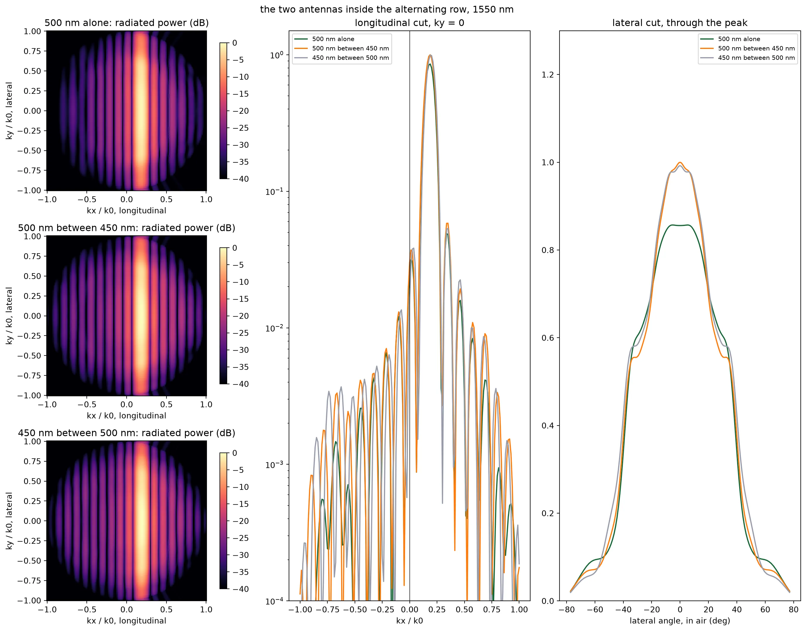

lateral angle   500 nm alone   500 nm in row   450 nm in row   (relative to the 500 nm alone peak)
     0 deg         1.00           1.17            1.16
    10 deg         0.98           1.09            1.10
    20 deg         0.82           0.81            0.84
    30 deg         0.71           0.65            0.68
    40 deg         0.40           0.44            0.49

antenna efficiency: 92 percent radiated over 1050 um, 48 percent of it reaching the air: 44 percent, 3.5 dB

The crosstalk is tens of decibels down, as the mode solver predicted for the detuned pair. The two antennas have patterns of the same shape, since the stack decides the shape and the strip width barely enters. Inside the row each pattern rises by about a fifth near normal, because the neighbouring strips catch part of the light that leaves sideways and send some of it back upward. The steering page uses these two patterns, one per width.

Step 6: from the simulated section to the real antenna

The simulated section is 15 um long and the antenna is a millimetre. Nothing about the cross-section changes along the antenna, so the lateral pattern is the same for the whole antenna as for the section. What changes is the longitudinal cut, the Fourier transform of the emitted amplitude along $x$ : the longer the emitter, the narrower the lobe. The guided power falls as $e^{-2\alpha x}$ , so the radiated amplitude falls as $e^{-\alpha x}$ , and over a length $L$

A(k_x) \propto \int_0^L e^{-\alpha x}\, e^{-j (k_x - k_{x0}) x}\, dx = \frac{1 - e^{-(\alpha + j\,\Delta k_x) L}}{\alpha + j\,\Delta k_x}.

For the section $\alpha L$ is a few hundredths and this is the $\mathrm{sinc}^2$ of a uniform aperture, which the measured longitudinal cut checks; for the antenna $\alpha L$ is 1.2 and the lobe is a tenth of a degree wide. The longitudinal beam is thus known from the length and the decay rate, without a millimetre-long FDTD run.

# wavenumber in the oxide, where the section's monitor sits
k_ox = 2 * np.pi * n_oxide / lda0
# the emission peak of the section's longitudinal cut
u_peak = float(u_grid[np.argmax(antenna["longitudinal"][:, i0])])

def longitudinal_lobe(length, ux_axis):
    """Longitudinal spectrum of an antenna of the given length, from the measured decay rate."""
    dk = k_ox * (ux_axis - u_peak)
    a = (1 - np.exp(-(antenna["alpha"] + 1j * dk) * length)) / (
        antenna["alpha"] + 1j * dk
    )
    return np.abs(a) ** 2

def width_deg(ux_axis, lobe):
    """Full width at half maximum of a lobe, in degrees of emission angle in air, on a fine grid."""
    fine = np.linspace(ux_axis.min(), ux_axis.max(), 40 * ux_axis.size)
    above = fine[np.interp(fine, ux_axis, lobe) > lobe.max() / 2]
    return np.degrees(
        np.arcsin(n_oxide * above.max()) - np.arcsin(n_oxide * above.min())
    )

measured_lobe = antenna["longitudinal"][:, i0] / antenna["longitudinal"][:, i0].max()
predicted = longitudinal_lobe(l_section, u_grid)
print(
    f"{l_section:.0f} um section: {width_deg(u_grid, measured_lobe):.2f} deg wide simulated, "
    f"{width_deg(u_grid, predicted / predicted.max()):.2f} deg from the formula"
)
ux_fine = np.linspace(u_peak - 0.01, u_peak + 0.01, 4001)
lobe_full = longitudinal_lobe(l_antenna, ux_fine)
print(
    f"{l_antenna:.0f} um antenna: {width_deg(ux_fine, lobe_full):.3f} deg wide, against lambda / L = "
    f"{np.degrees(lda0 / l_antenna):.3f} deg for a uniform emitter of the same length"
)

# Wavelength steering of the section, against the grating equation with the measured index
n_avg_lda = n_avg_chosen + (n_eff_lda - n_eff_strip)
theta_expected = np.degrees(np.arcsin(n_avg_lda - wavelengths / period_chosen))
peak_angle = antenna["angles"]
slope_fdtd = np.polyfit(wavelengths * 1e3, peak_angle, 1)[0]
print(
    f"wavelength steering {slope_fdtd:.3f} deg/nm simulated, {np.polyfit(wavelengths * 1e3, theta_expected, 1)[0]:.3f} deg/nm "
    f"from the grating equation, {abs(slope_fdtd) * (wavelengths[-1] - wavelengths[0]) * 1e3:.1f} deg over the tune"
)

fig, ax = plt.subplots(1, 2, figsize=(11, 4))
theta_ox = np.degrees(np.arcsin(np.clip(n_oxide * u_grid, -1, 1)))
ax[0].plot(theta_ox, measured_lobe, label=f"FDTD, {l_section:.0f} um section")
ax[0].plot(
    theta_ox, predicted / predicted.max(), "--", label=f"formula, {l_section:.0f} um"
)
ax[0].plot(
    np.degrees(np.arcsin(n_oxide * ux_fine)),
    lobe_full / lobe_full.max(),
    label=f"formula, {l_antenna:.0f} um",
)
ax[0].set_xlim(theta0 - 12, theta0 + 12)
ax[0].set_xlabel("longitudinal angle, in air (deg)")
ax[0].set_ylabel("radiated power (normalized)")
ax[0].set_title("longitudinal lobe: section and full antenna")
ax[0].legend(fontsize=8)
for i, lda in enumerate(wavelengths):
    (line,) = ax[1].plot(
        theta_ox,
        antenna["longitudinal"][:, i] / antenna["longitudinal"].max(),
        label=f"{lda * 1e3:.0f} nm",
    )
    ax[1].axvline(
        theta_expected[i], color=line.get_color(), linestyle="--", linewidth=0.8
    )
ax[1].set_xlim(theta0 - 12, theta0 + 12)
ax[1].set_xlabel("longitudinal angle, in air (deg)")
ax[1].set_title("wavelength steering, grating equation dashed")
ax[1].legend(fontsize=8)
plt.tight_layout()
plt.show()

# The later pages read this file: the patterns and the antenna numbers
theta_500, lateral_500, _ = embedded["500 nm between 450 nm"]
theta_450, lateral_450, _ = embedded["450 nm between 500 nm"]
np.savez(
    "misc/element_far_field.npz",
    ux=alone["ux"],
    uy=alone["uy"],
    spectrum=alone["power"],
    theta_lateral=alone["theta"],
    lateral=alone["lateral"],
    theta_500=theta_500,
    lateral_500=lateral_500,
    theta_450=theta_450,
    lateral_450=lateral_450,
    theta_lateral_alt=measured[alternative]["theta"],
    lateral_alt=measured[alternative]["lateral"],
    alternative=alternative,
    wavelengths=wavelengths,
    peak_angle=peak_angle,
    alpha=antenna["alpha"],
    alpha_second=design[width_second]["result"]["alpha"],
    to_air=alone["to_air"],
    efficiency=efficiency,
    period=period_chosen,
    period_second=design[width_second]["period"],
    tooth=tooth,
    duty=duty_chosen,
    duty_second=design[width_second]["duty"],
    width_second=width_second,
    l_antenna=l_antenna,
    pitch=pitch,
)
print("saved misc/element_far_field.npz")

14 um section: 5.83 deg wide simulated, 5.86 deg from the formula
1050 um antenna: 0.080 deg wide, against lambda / L = 0.085 deg for a uniform emitter of the same length
wavelength steering -0.158 deg/nm simulated, -0.151 deg/nm from the grating equation, 6.3 deg over the tune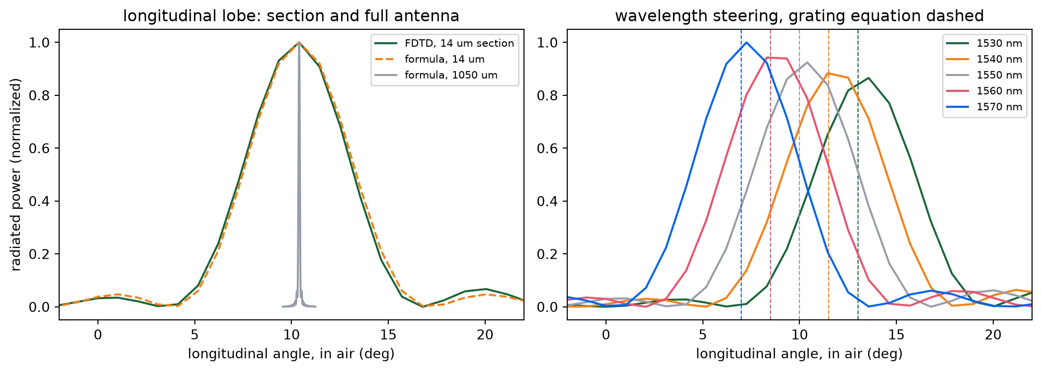

saved misc/element_far_field.npz

The formula reproduces the lobe of the section, so it can be used for the antenna, which is too long to simulate. The lobe of the full antenna is a little narrower than the $\lambda/L$ of a uniform emitter, because the decaying amplitude weights the near end. It keeps small sidelobes because the far end still carries 30 percent of the amplitude where the antenna ends. Tuning the laser by 40 nm moves the emission by six degrees, at the rate the grating equation predicts. That is the second steering axis.

What the later pages take

Two antenna cells with their periods and duty cycles, the antenna length, the decay rates the layout page turns into radiating waveguide models, the antenna efficiency the budget carries, and the two patterns the steering page multiplies by the array factor. The component library builds everything else the chip needs.