

Waveguide Coupling Simulation with Port Bending
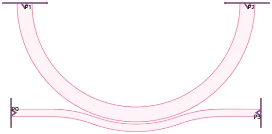
In this notebook, we will:
- Create a waveguide coupled to a multi-mode waveguide, using a pulley coupler.
- Incorporate port bending radius into the simulation.
- Perform an S-matrix simulation and calculate the coupling efficiency.
import numpy as npimport photonforge as pfimport tidy3d as tdfrom matplotlib import pyplot as plt
td.config.logging.level = "ERROR"
We will use the SiEPIC OpenEBL through the siepic_forge module. So, we set up the default photonic technology, simulation mesh refinement, and define the wavelength range for our simulations from 1.53 µm to 1.57 µm.
import siepic_forge as siepic
tech = siepic.ebeam()
pf.config.default_technology = techpf.config.default_mesh_refinement = 12.0wavelengths = np.linspace(1.53, 1.57, 51)
Next, we define the waveguide ports for our simulation. We start by using a default siepic waveguide port specification (“TE_1550_500”). Then, we create a new custom port specification for a wider multi-mode waveguide.
The new multi-mode waveguide (port_spec_mm) has the following properties:
- Port width: 3 µm
- Number of modes: 2 (multi-mode)
- Target effective index (
target_neff): 3.5 - Port limits in the z direction: (-1, 1.22)
# The default narrow waveguideport_spec = tech.ports["TE_1550_500"]
# You can create new port spec for a wider multi-mode waveguide like thismm_wg_width = 1port_spec_mm = pf.PortSpec(    description="Multi mode strip",    width=3,    num_modes=2,    target_neff=3.5,    limits=(-1, 1.22),    path_profiles=[(mm_wg_width, 0, (1, 0))],)
After defining a new port, it’s important to verify that its mode properties are correctly computed. Specifically, we must confirm that the mode field fully decays at the port boundaries. If the mode hasn’t adequately decayed, it is necessary to increase the width and limits parameters of the port.
We first calculate the mode at the default “TE_1550_500” port as a benchmark, and then we compare it with the modes calculated at the newly defined port.
Mode for the single mode port
Section titled “Mode for the single mode port”First, we calculate the guided modes at port “TE_1550_500” using a dedicated mode solver. The calculation is performed at the reference wavelength of 1.55 µm, with a refined mesh (mesh_refinement=40) to achieve accurate mode profiles.
The resulting mode properties are presented clearly in a pandas data frame for convenient inspection.
mode_solver = pf.port_modes(    port_spec,    frequencies=[pf.C_0 / 1.55],    mesh_refinement=40,    group_index=True,)
mode_solver.data.to_dataframe()
Uploading task 'Mode-ModeSolver…'Starting task 'Mode-ModeSolver': https://tidy3d.simulation.cloud/workbench?taskId=mo-2448784a-3cd1-44ad-ab25-363b07beb31dDownloading data from 'Mode-ModeSolver'…| wavelength | n eff | k eff | loss (dB/cm) | TE (Ey) fraction | wg TE fraction | wg TM fraction | mode area | group index | dispersion (ps/(nm km)) | ||
|---|---|---|---|---|---|---|---|---|---|---|---|
| f | mode_index | ||||||||||
| 1.934145e+14 | 0 | 1.55 | 2.442662 | 0.0 | 0.0 | 0.983483 | 0.763836 | 0.817709 | 0.190931 | 4.186253 | 508.873435 |
Here, we visualize the electric field (E-field) distribution of the fundamental mode (mode index 0) at the port “TE_1550_500” for the reference wavelength of 1.55 µm.
_ = mode_solver.plot_field("E", mode_index=0, f=pf.C_0 / 1.55)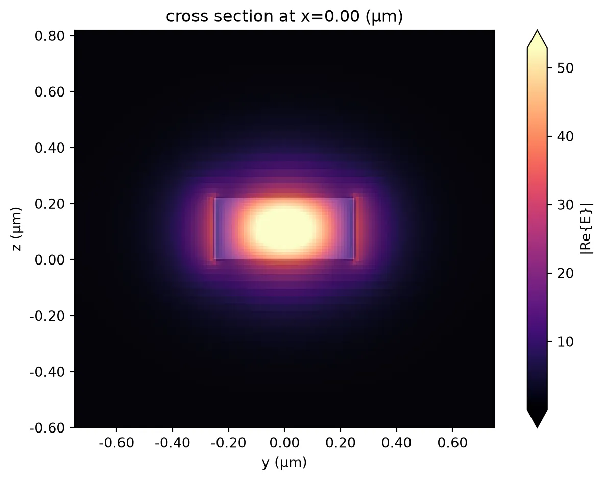
Modes for the multi-mode port
Section titled “Modes for the multi-mode port”Similarly, we compute the guided modes at the multi-mode port.
mode_solver_mm = pf.port_modes(    port_spec_mm,    frequencies=[pf.C_0 / 1.55],    mesh_refinement=40,    group_index=True,)
mode_solver_mm.data.to_dataframe()
Uploading task 'Mode-ModeSolver…'Starting task 'Mode-ModeSolver': https://tidy3d.simulation.cloud/workbench?taskId=mo-11e0a4d9-6990-410f-920b-f61c4feb1682Downloading data from 'Mode-ModeSolver'…| wavelength | n eff | k eff | loss (dB/cm) | TE (Ey) fraction | wg TE fraction | wg TM fraction | mode area | group index | dispersion (ps/(nm km)) | ||
|---|---|---|---|---|---|---|---|---|---|---|---|
| f | mode_index | ||||||||||
| 1.934145e+14 | 0 | 1.55 | 2.742640 | 0.0 | 0.0 | 0.998382 | 0.929515 | 0.804931 | 0.234369 | 3.827183 | -802.324232 |
| 1 | 1.55 | 2.416388 | 0.0 | 0.0 | 0.988951 | 0.738582 | 0.835732 | 0.332785 | 4.280778 | 1602.044386 |
_, ax = plt.subplots(1, 2, figsize=(10, 3.5), tight_layout=True)_ = mode_solver_mm.plot_field("E", mode_index=0, f=pf.C_0 / 1.55, ax=ax[0])_ = mode_solver_mm.plot_field("E", mode_index=1, f=pf.C_0 / 1.55, ax=ax[1])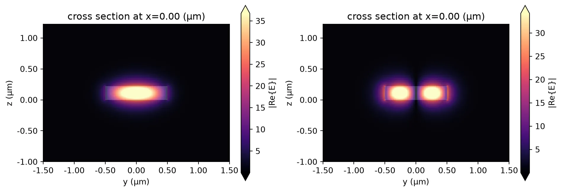
It is evident that the fields have fully decayed at the port boundaries, confirming that the current port dimensions are sufficient (you can set scale="dB" in the plots to confirm the decay).
Defining the Pulley Coupler Component
Section titled “Defining the Pulley Coupler Component”We define the function make_pulley_coupler to construct a photonic pulley coupler component. This function generates a coupler comprising a ring waveguide coupled to a bus waveguide. Parameters such as the ring radius, coupling angle, and gap size between waveguides can be customized. Additionally, the waveguide port specifications are defined through the inputs port_spec_bus and port_spec_ring.
def make_pulley_coupler(    ring_radius=7.5,    coupling_angle=20,    gap=0.15,    port_spec_bus=port_spec,    port_spec_ring=port_spec_mm,):    # Error check    if coupling_angle > 70:        raise ValueError("Coupling angle cannot be greater than 70 degrees.")
    if isinstance(port_spec_bus, str):        port_spec_bus = pf.config.default_technology.ports[port_spec_bus]
    if isinstance(port_spec_ring, str):        port_spec_ring = pf.config.default_technology.ports[port_spec_ring]
    c = pf.Component("Pulley Coupler")
    # Extract waveguide widths from port specifications    bus_width = port_spec_bus.path_profiles[0][0]  # Bus waveguide width (single-mode)    ring_width = port_spec_ring.path_profiles[0][0]  # Ring waveguide width (multimode)
    # Bus waveguide bending radius calculation    bus_radius = ring_radius + ring_width / 2 + gap + bus_width / 2
    # Calculate input coordinates for bus waveguide    x_in = -bus_radius * np.sin(np.radians(coupling_angle))    y_in = -bus_radius * np.cos(np.radians(coupling_angle))
    # Define bus input path based on coupling angle    if coupling_angle < 30:        bus = pf.Path((-bus_radius, 2 * y_in + bus_radius), bus_width)        bus.segment((2 * x_in, 2 * y_in + bus_radius))        bus.turn(-coupling_angle, radius=bus_radius)        bus.turn(2 * coupling_angle, radius=bus_radius)        bus.turn(-coupling_angle, radius=bus_radius)        bus.segment((bus_radius, 2 * y_in + bus_radius))    else:        bus = pf.Path((2 * x_in, 2 * y_in + bus_radius), bus_width)        bus.turn(-coupling_angle, radius=bus_radius)        bus.turn(2 * coupling_angle, radius=bus_radius)        bus.turn(-coupling_angle, radius=bus_radius)
    # Create ring waveguide    ring = pf.Circle(        radius=ring_radius + ring_width / 2,        inner_radius=ring_radius - ring_width / 2,        sector=(-180, 0),    )
    # Add waveguide elements to the component    c.add("Si", bus, ring)
    # Detect and add ports    c.add_port(c.detect_ports([port_spec_bus, port_spec_ring]))    assert len(c.ports) == 4, "Port detection failed: expected exactly 4 ports."
    # Assign a bend radius to both ring ports    c["P1"].bend_radius = ring_radius    c["P2"].bend_radius = -ring_radius
    # Finally, add a Tidy3D model to calculate S parameters.    c.add_model(pf.Tidy3DModel(), "Tidy3D")
    return c
# Create coupler with specified ring radiusring_radius = 7.5coupler = make_pulley_coupler(ring_radius=ring_radius)coupler
To verify the created component, we print out the available ports using a simple loop. Each port’s key and corresponding properties are displayed, allowing easy inspection and verification before simulation or further layout generation.
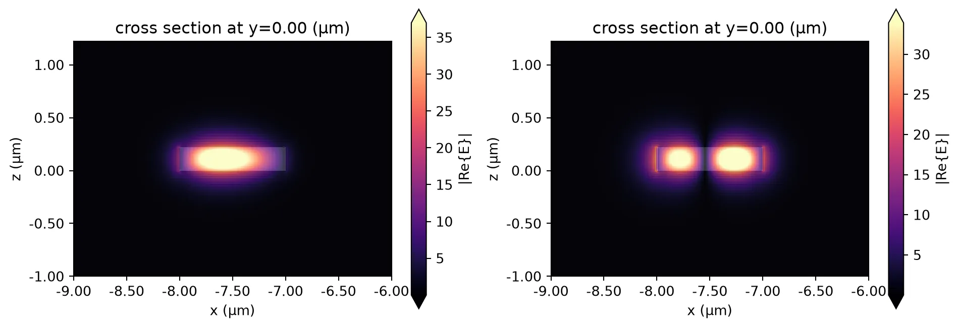
for name, port in coupler.ports.items(): print(f"{name}: {port}")P0: Port at (-8.4, -7.387) at 0 deg with spec "Strip TE 1550 nm, w=500 nm"P1: Port at (-7.5, 0) at 270 deg with spec "Multi mode strip"P2: Port at (7.5, 0) at 270 deg with spec "Multi mode strip"P3: Port at (8.4, -7.387) at 180 deg with spec "Strip TE 1550 nm, w=500 nm"It is important to note that the ring ports are set with a proper bend radius that follows the ring curvature. If we inspect the modes at the port and compare to the ones calculated previously directly from the multi-mode port specification (without bend radius), we can clearly see the differences:
mode_solver_p1 = pf.port_modes(    coupler["P1"],    frequencies=[pf.C_0 / 1.55],    mesh_refinement=40,    group_index=True,)
_, ax = plt.subplots(1, 2, figsize=(10, 3.5), tight_layout=True)_ = mode_solver_p1.plot_field("E", mode_index=0, f=pf.C_0 / 1.55, ax=ax[0])_ = mode_solver_p1.plot_field("E", mode_index=1, f=pf.C_0 / 1.55, ax=ax[1])
mode_solver_p1.data.to_dataframe()
Uploading task 'Mode-ModeSolver…'Starting task 'Mode-ModeSolver': https://tidy3d.simulation.cloud/workbench?taskId=mo-3edd669f-e77a-4fec-8fff-22dede32ae30Downloading data from 'Mode-ModeSolver'…| wavelength | n eff | k eff | loss (dB/cm) | TE (Ex) fraction | wg TE fraction | wg TM fraction | mode area | group index | dispersion (ps/(nm km)) | ||
|---|---|---|---|---|---|---|---|---|---|---|---|
| f | mode_index | ||||||||||
| 1.934145e+14 | 0 | 1.55 | 2.756291 | 0.0 | 0.0 | 0.997773 | 0.921479 | 0.805650 | 0.227045 | 3.880552 | -1111.172148 |
| 1 | 1.55 | 2.411001 | 0.0 | 0.0 | 0.988632 | 0.741699 | 0.835644 | 0.325203 | 4.259365 | 1609.693557 |
Coupling Calculation
Section titled “Coupling Calculation”Next, we compute the S-parameters (scattering parameters) specifically for the input port “P0”. This calculation characterizes the coupler’s transmission and reflection behavior over the previously defined wavelength range.
s_matrix = coupler.s_matrix(pf.C_0 / wavelengths, model_kwargs={"inputs": ["P0"]})Uploading task 'P0@0…'Starting task 'P0@0': https://tidy3d.simulation.cloud/workbench?taskId=fdve-c2b2f06b-e72c-4f0b-801e-8b9700cc9f8aDownloading data from 'P0@0'…We visualize the computed S-parameters using plot_s_matrix. We observe approximately 4.2% power transfer from the bus waveguide into the ring waveguide’s fundamental mode and about 1.3% coupling into the second mode.
_ = pf.plot_s_matrix(s_matrix)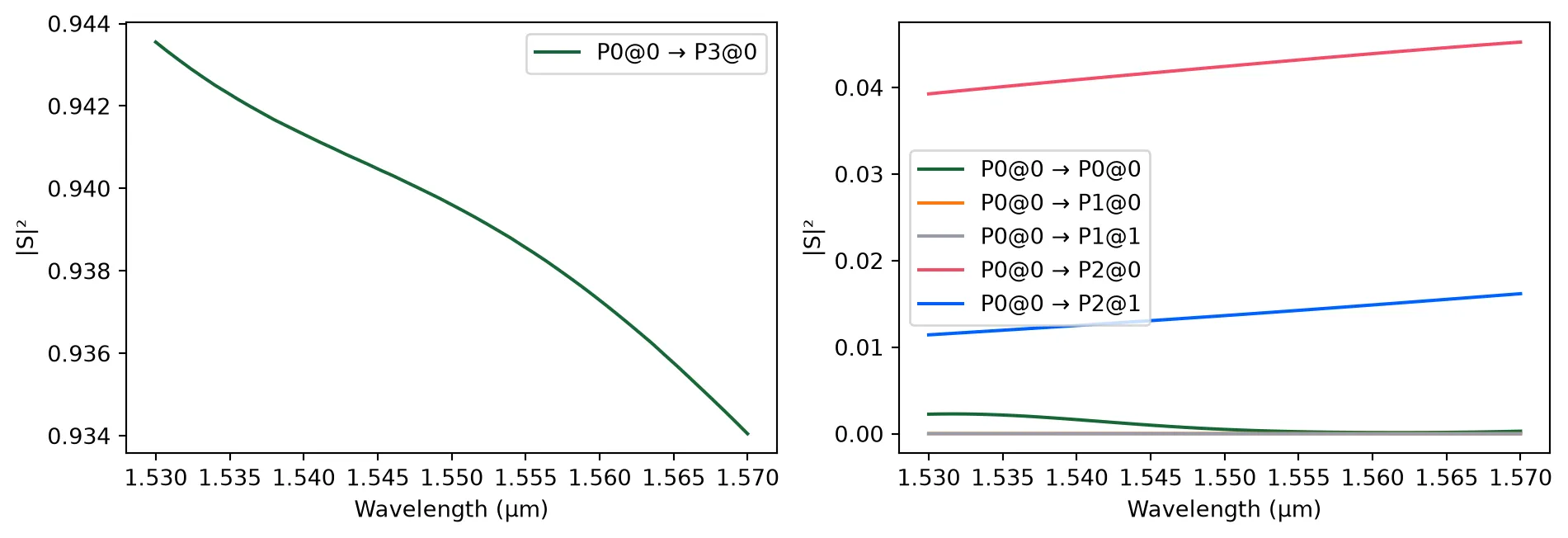
For comparison, we can remove the bend radius from the ring ports and see the changes in coupling:
straight_port_coupler = make_pulley_coupler(ring_radius=ring_radius)straight_port_coupler["P1"].bend_radius = 0straight_port_coupler["P2"].bend_radius = 0straight_port_coupler
straight_port_s_matrix = straight_port_coupler.s_matrix(    pf.C_0 / wavelengths, model_kwargs={"inputs": ["P0@0"]})
_ = pf.plot_s_matrix(straight_port_s_matrix)
Uploading task 'P0@0…'Starting task 'P0@0': https://tidy3d.simulation.cloud/workbench?taskId=fdve-46b09a6f-1fa1-4e00-9874-8d514a34db89Downloading data from 'P0@0'…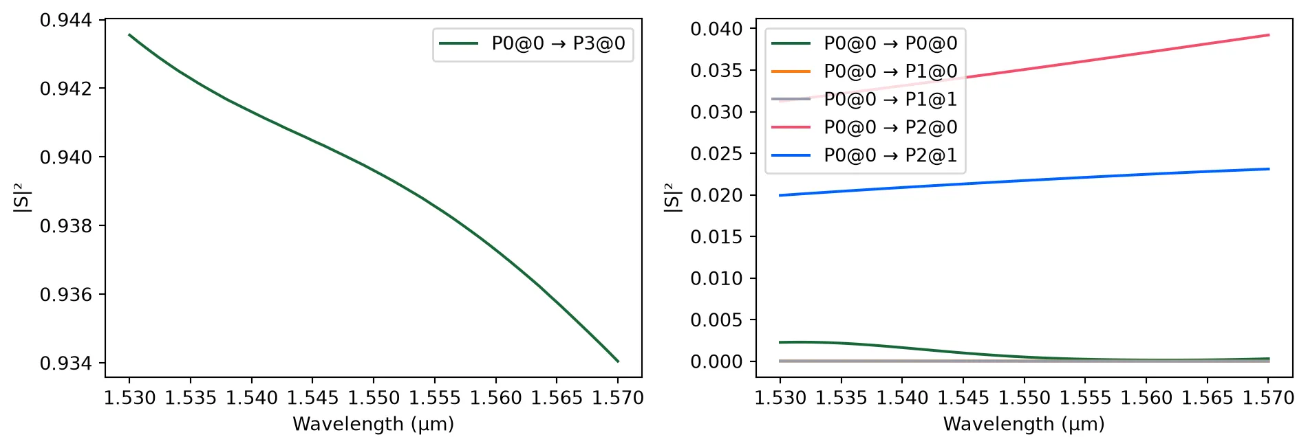
We can plot both results together to see the differences more clearly:
_, ax = plt.subplots(1, 2, figsize=(10, 3.5), tight_layout=True)
# Through port comparisonthru_bend = np.abs(s_matrix["P0@0", "P3@0"]) ** 2thru_straight = np.abs(straight_port_s_matrix["P0@0", "P3@0"]) ** 2
ax[0].plot(wavelengths, thru_bend, label="with bend")ax[0].plot(wavelengths, thru_straight, label="straight")
# Through port comparisondrop_bend = np.abs(s_matrix["P0@0", "P2@0"]) ** 2drop_straight = np.abs(straight_port_s_matrix["P0@0", "P2@0"]) ** 2
ax[1].plot(wavelengths, drop_bend, label="with bend")ax[1].plot(wavelengths, drop_straight, label="straight")
ax[0].set(xlabel="Wavelength (μm)", ylabel="Thru port transmission")ax[1].set(xlabel="Wavelength (μm)", ylabel="Drop port transmission")
ax[0].legend()_ = ax[1].legend()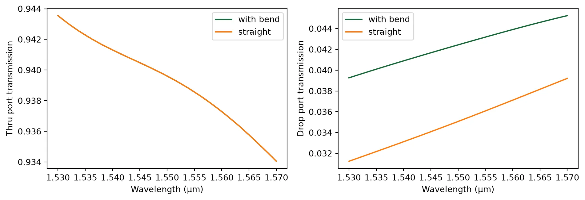
As expected, the transmitted power to port “P3” (thru port) remains unchanged, since no bending adjustments were applied to this port. However, when bending effects are removed from port “P2” (drop port), we observe a reduction in the coupled power to that port mode.