Nonlinear Waveguide

Download notebook (.zip)

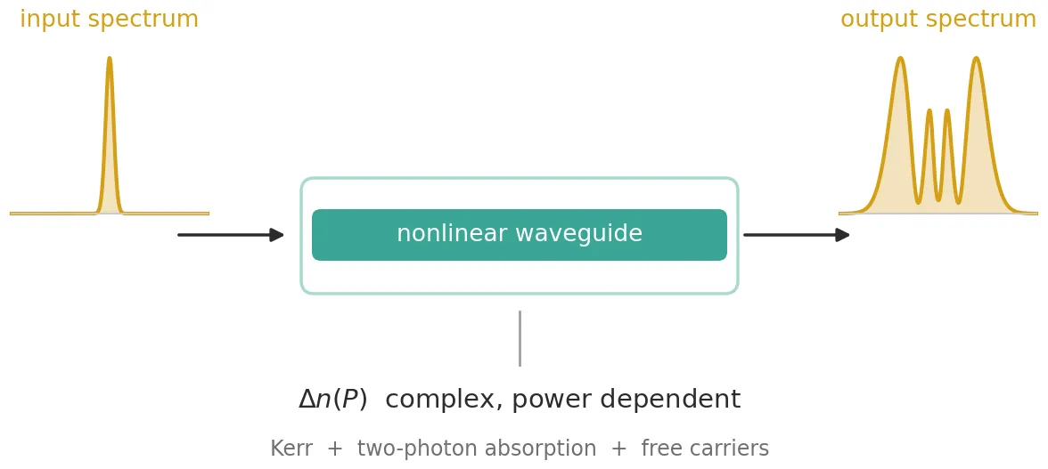
AnalyticWaveguideTimeStepper is the time-domain model of a waveguide. Besides the linear properties it shares with AnalyticWaveguideModel, namely the effective index, group index, propagation loss and chromatic dispersion, it accepts an effective index that depends on the optical power in the guide. That makes it a model of a nonlinear waveguide.

The class method AnalyticWaveguideModel.nonlinear builds such a model from physical parameters: the Kerr coefficient, the two-photon absorption coefficient, the free-carrier coefficients and the waveguide cross-section. The model it returns works both on an abstract black box and on a real layout, such as a routed spiral, whose length it reads from the geometry. This guide uses it for a silicon wire, where the power-dependent index comes from the Kerr effect, two-photon absorption and the free carriers that two-photon absorption creates.

What the time stepper computes

The stepper propagates the complex envelope $A(t)$ of the optical field, normalised so that $P(t) = \lvert A(t) \rvert^2$ is the optical power in watts. The oscillation at the carrier frequency $f_c$ is removed from the signal and handled by the stepper. Over a length $L$, a change $\delta n$ of the effective index multiplies the envelope by

$$A_\mathrm{out} = A_\mathrm{in}\, e^{i k_0\, \delta n\, L}, \qquad k_0 = \frac{2\pi}{\lambda},$$

on top of the linear delay and loss, where $\lambda$ is the vacuum wavelength. Writing $\delta n = \delta n' + i\,\delta n''$ separates two effects:

• the real part $\delta n'$ adds a phase $\phi = k_0\,\delta n'\,L$;
• the imaginary part $\delta n''$ attenuates the power as $e^{-\alpha L}$, with an added absorption coefficient $\alpha = 2 k_0\,\delta n'' = 4\pi\,\delta n''/\lambda$.

A single complex $\delta n$ therefore describes both a phase change and a loss. The stepper sums three contributions, each set by one of its parameters:

• dn_kerr sets an index change that follows the power instantly, $\delta n_\mathrm{K}(t) = \Delta n_\mathrm{K}\big(P(t)\big)$.

• dn_fc sets the free-carrier contribution. A quantity $x$ relaxes towards its steady-state value with the time constant tau_fc,

  $$\tau_\mathrm{fc}\,\frac{\mathrm{d}x}{\mathrm{d}t} + x = x_\mathrm{ss}\big(P(t)\big),$$

  and $x$ is either the index change itself or, when dn_fc_map is given, the carrier density, which the map then converts to an index change.

• dn_th sets a second relaxing index change with the time constant tau_th, intended for heating. It is not used in this guide.

Each of these is a complex Interpolator against power. A relaxing channel settles at its steady state after a few time constants under constant power, and responds to the power averaged over roughly one time constant when the power changes faster than that.

The stepper also splits the waveguide into sections. Each section applies its nonlinear phase at the power entering it, so the phase, the loss and the dispersion alternate along the length in small steps, which is the split-step method. With peak_power given, the number of sections is chosen so that the Kerr phase per section stays below max_phase, 0.05 rad by default.

Nonlinear optics of a silicon wire

At 1550 nm four effects change the index of a silicon waveguide. All of them depend on the intensity $I = P/A_\mathrm{eff}$, where $A_\mathrm{eff}$ is the nonlinear effective area of the mode.

Kerr effect. The electronic response of silicon raises the refractive index in proportion to the intensity, $\Delta n = n_2 I$, where $n_2$ is the Kerr coefficient. The response takes femtoseconds, so it is instantaneous for picosecond pulses. A pulse whose power varies in time therefore acquires a phase that varies in time. This is self-phase modulation (SPM): the pulse becomes chirped and its spectrum broadens.

Two-photon absorption (TPA). A 1550 nm photon carries 0.8 eV, less than the 1.12 eV bandgap of silicon. One photon cannot be absorbed, but two photons together can. The absorption grows with intensity, $\mathrm{d}I/\mathrm{d}z = -\beta_\mathrm{TPA} I^2$, which is an absorption coefficient $\alpha = \beta_\mathrm{TPA} I$. With $\alpha = 4\pi\,\delta n''/\lambda$ this is an imaginary index $\delta n'' = \lambda\,\beta_\mathrm{TPA} I/(4\pi)$. TPA is as fast as the Kerr effect, so both go on dn_kerr.

Free carriers. Each two-photon absorption creates one electron-hole pair. The absorbed power per unit volume is $\beta_\mathrm{TPA} I^2$, and each pair uses two photons of energy $h\nu$, where $h$ is the Planck constant and $\nu$ the optical frequency. The carrier density $N$ therefore obeys the rate equation

$$\frac{\mathrm{d}N}{\mathrm{d}t} = \frac{\beta_\mathrm{TPA} I^2}{2h\nu} - \frac{N}{\tau_c},$$

where $\tau_c$ is the carrier lifetime, about 1 ns in a silicon wire. Multiplying by $\tau_c$ gives

$$\tau_c\,\frac{\mathrm{d}N}{\mathrm{d}t} + N = N_\mathrm{ss}, \qquad N_\mathrm{ss} = \frac{\tau_c\,\beta_\mathrm{TPA}}{2h\nu}\,I^2,$$

which is exactly the relaxation equation of dn_fc, with tau_fc equal to the carrier lifetime and $N_\mathrm{ss}$ the steady-state density under constant intensity. The carriers change the index in two ways:

• free-carrier absorption (FCA): the carriers absorb light with $\alpha = \sigma_a N$, where $\sigma_a$ is the absorption cross section of electrons and holes together;
• free-carrier dispersion (FCD): the carriers lower the refractive index. The measured dependence of Soref and Bennett is $\Delta n = c_e N^{e_e} + c_h N^{e_h}$, with $e_e = 1$ for electrons and $e_h = 0.8$ for holes, and $c_e, c_h < 0$.

When the index change is proportional to $N$, relaxing the index change is the same as relaxing $N$. The hole term of Soref and Bennett is not proportional, so the carrier density itself must relax and be converted afterwards: that is what dn_fc_map does, and the class method uses it whenever an exponent differs from one.

Effective area. In a high-index-contrast wire the mode is not a plane wave, and the effective area is defined from the Kerr response integrated over the cross-section, normalised by the power the mode carries:

$$\frac{n_2}{A_\mathrm{eff}} = \frac{\int n^2\, n_2\, \left(2\lvert E \rvert^4 + \lvert E\cdot E \rvert^2\right)/3\;\mathrm{d}S} {Z_0^2 \left(\int \mathrm{Re}(E\times H^*)\cdot\hat{z}\;\mathrm{d}S\right)^2},$$

where $Z_0$ is the impedance of free space and $n_2$ is non-zero only in the nonlinear material. The class method evaluates this integral from a mode solve when it is given the cross-section.

The four effects map onto the two channels as follows:

effect	index change $\Delta n(P)$	channel
Kerr effect	$n_2 I$	dn_kerr
two-photon absorption	$i\,\lambda\,\beta_\mathrm{TPA} I/(4\pi)$	dn_kerr
free-carrier dispersion	$c_e N^{e_e} + c_h N^{e_h}$	dn_fc, with tau_fc $=\tau_c$
free-carrier absorption	$i\,\lambda\,\sigma_a N/(4\pi)$	dn_fc, with tau_fc $=\tau_c$

The first part of the guide uses the 2 cm silicon wire of Yin and Agrawal, with its parameters given explicitly, because their closed-form solution for SPM with TPA can be plotted for comparison. It shows what each effect does to a picosecond pulse and ends with chromatic dispersion acting on a femtosecond pulse. The last part builds a routed silicon spiral and lets the class method take every cross-section parameter from its port specification.

References

1. Yin, Lianghong and Agrawal, Govind P. “Impact of two-photon absorption on self-phase modulation in silicon waveguides.” Optics Letters 2007 32 (14), 2031-2033, doi: 10.1364/OL.32.002031.
2. Soref, Richard A. and Bennett, Brian R. “Electrooptical effects in silicon.” IEEE Journal of Quantum Electronics 1987 23 (1), 123-129, doi: 10.1109/JQE.1987.1073206.
3. Afshar V., Shahraam and Monro, Tanya M. “A full vectorial model for pulse propagation in emerging waveguides with subwavelength structures part I: Kerr nonlinearity.” Optics Express 2009 17 (4), 2298-2318, doi: 10.1364/OE.17.002298.
4. Agrawal, Govind P. Nonlinear Fiber Optics, 5th ed. Academic Press, 2013.

Setup

The parameters are those of the silicon wire of Yin and Agrawal: a 2 cm waveguide with 1 dB/cm linear loss, a nonlinear effective area of 0.1 µm², and the nonlinear coefficients of silicon at 1550 nm. The class method takes the material coefficients in SI units, as RingTimeStepper does, and lengths in µm, as the rest of PhotonForge.

Two names come from photonforge.utils: C_0, the speed of light in vacuum in µm/s, and virtual_port_spec, which creates ports without a physical cross-section for the abstract waveguide. The live viewer is opened here for the spiral at the end.

A few combinations of the parameters appear throughout. The loss in dB/µm is converted to a power attenuation coefficient $\alpha$ in 1/m. Because the power decays along the waveguide, the nonlinear effects act over the effective length

$$L_\mathrm{eff} = \frac{1 - e^{-\alpha L}}{\alpha},$$

which is shorter than $L$. The nonlinear coefficient $\gamma = k_0 n_2/A_\mathrm{eff}$ is the Kerr phase per watt of power and per metre of waveguide.

import matplotlib.pyplot as plt
import numpy as np
import photonforge as pf
import tidy3d as td
from photonforge.live_viewer import LiveViewer
from photonforge.utils import C_0, virtual_port_spec

# Open the live viewer for the layout at the end of the guide
viewer = LiveViewer()

# Use the basic technology for the abstract waveguide
pf.config.default_technology = pf.basic_technology()

# Set the figure resolution and a light grid for all plots
plt.rcParams.update({"figure.dpi": 110, "axes.grid": True, "grid.alpha": 0.3})

# Set the operating wavelength and the carrier frequency
wavelength = 1.55  # Vacuum wavelength (um)
carrier_frequency = C_0 / wavelength  # Optical carrier frequency (Hz)

# Set the linear properties of the silicon wire
length = 2.0e4  # Waveguide length: 2 cm (um)
n_eff = 2.45  # Effective index
n_group = 4.2  # Group index, which sets the delay
loss = 1.0 / 1e4  # Propagation loss: 1 dB/cm (dB/um)
area = 0.1e-12  # Nonlinear effective area: 0.1 um^2 (m^2)

# Set the nonlinear coefficients of silicon at 1550 nm
kerr_index = 6e-18  # Kerr coefficient n2 (m^2/W)
tpa = 5e-12  # Two-photon absorption coefficient beta_TPA (m/W)
fca = 1.45e-21  # Free-carrier absorption cross section sigma_a (m^2)
fcd = -1.35e-27  # Index change per carrier density, linear in N (m^3)
carrier_lifetime = 1e-9  # Carrier lifetime tau_c (s)

# Compute the vacuum wavenumber (1/m)
k0 = 2 * np.pi / (wavelength * 1e-6)

# Convert the loss from dB/um to a power attenuation coefficient (1/m)
alpha = loss * 1e6 * np.log(10) / 10

# Compute the effective length over which the nonlinear effects act (m)
l_eff = (1 - np.exp(-alpha * length * 1e-6)) / alpha

# Compute the nonlinear coefficient gamma = k0 n2 / A_eff (1/(W m))
gamma = k0 * kerr_index / area

# Print the derived quantities
print(
    f"alpha = {alpha:.2f} 1/m, effective length = {l_eff * 1e3:.2f} mm, "
    f"gamma = {gamma:.0f} 1/(W m)"
)

LiveViewer started at http://127.0.0.1:44871. Call its 'stop()' method to free the port.
alpha = 23.03 1/m, effective length = 16.03 mm, gamma = 243 1/(W m)

Creating the nonlinear waveguide model

pf.AnalyticWaveguideModel.nonlinear returns an AnalyticWaveguideModel for frequency-domain simulations with an AnalyticWaveguideTimeStepper attached as its time_stepper. Its arguments are the physical parameters:

• the cross-section: n_eff, n_group, dispersion and effective_area, given here explicitly;
• the waveguide: length and propagation_loss;
• the material: kerr_index, tpa_coefficient, fca_cross_section, fcd_coefficients $(c_e, c_h)$, fcd_exponents $(e_e, e_h)$ and carrier_lifetime;
• the discretisation: peak_power, the highest power expected at the input, from which the number of sections follows.

From these it builds the interpolators of the stepper, exact at every power:

• dn_kerr is linear in power, so two samples define it everywhere;
• the steady-state free-carrier term grows as $P^2$, so three samples of a "cubicspline" interpolator define it everywhere: through three samples, the spline is the parabola itself;
• tau_fc is the carrier lifetime.

The function below wraps the class method in a parametric component, so that each comparison switches effects on and off with one argument. With the free carriers off, the carrier lifetime is zero, which disables the channel. The model is turned into a black box with virtual ports.

@pf.parametric_component
def silicon_wire(
    *,
    peak_power=0.0,
    kerr=True,
    tpa_on=True,
    carriers=False,
    fcd_on=True,
    dispersion=0.0,
    linear_loss=True,
    total_length=length,
    sections=None,
):
    """Silicon wire of Yin and Agrawal, with the chosen nonlinear effects active."""
    # Create the model and its nonlinear time stepper from the physical parameters
    model = pf.AnalyticWaveguideModel.nonlinear(
        reference_frequency=carrier_frequency,
        n_eff=n_eff,
        n_group=n_group,
        dispersion=dispersion,
        effective_area=area,
        length=total_length,
        propagation_loss=loss if linear_loss else 0.0,
        kerr_index=kerr_index if kerr else 0.0,
        tpa_coefficient=tpa if tpa_on else 0.0,
        fca_cross_section=fca,
        fcd_coefficients=(fcd if fcd_on else 0.0, 0.0),
        carrier_lifetime=carrier_lifetime if carriers else 0.0,
        peak_power=peak_power,
        sections=sections,
    )

    # Create a two-port black box carrying the model
    return model.black_box_component(virtual_port_spec(), name="Silicon wire")

def propagate(waveguide, pulse, time_step):
    """Step a pulse envelope through a waveguide and return the output envelope."""
    # Set up the time stepper for this time step and carrier frequency
    stepper = waveguide.setup_time_stepper(
        time_step, carrier_frequency, show_progress=False
    )

    # Inject the pulse at the input port and step through the whole record
    inputs = pf.TimeSeries({"P0@0": pulse}, time_step)
    output = stepper.step(inputs=inputs, show_progress=False)

    # Return the envelope at the output port
    return output["P1@0"]

Before any pulse is launched, the interpolators of the stepper can be plotted to compare the size of each effect. They are read from the parametric_kwargs of the time stepper. On logarithmic axes the linear and quadratic power laws appear as straight lines of slope one and two. The imaginary parts are converted to an absorption coefficient in 1/cm, $\alpha = 4\pi\,\delta n''/\lambda$, and compared with the 1 dB/cm linear loss.

# Create the wire with every effect on and read its stepper's interpolators
wire = silicon_wire(carriers=True)
tables = wire.active_model.time_stepper.parametric_kwargs

# Evaluate both channels from 1 mW to 20 W
plot_powers = np.logspace(-3, np.log10(20.0), 400)
kerr_values = tables["dn_kerr"](plot_powers)
carrier_values = tables["dn_fc"](plot_powers)

# Set the factor that converts an imaginary index into an absorption coefficient (1/cm)
to_per_cm = 4 * np.pi / (wavelength * 1e-6) / 100

# Create two panels, for the real and the imaginary parts
fig, axes = plt.subplots(1, 2, figsize=(10, 3.5), tight_layout=True)

# Plot the real parts as magnitudes, since the Kerr change is positive and FCD negative
axes[0].loglog(plot_powers, kerr_values.real, label="Kerr (positive)")
axes[0].loglog(
    plot_powers, -carrier_values.real, label="free-carrier dispersion (negative)"
)
axes[0].set_ylabel(r"magnitude of real $\Delta n$")
axes[0].set_ylim(1e-9, 1e1)

# Plot the absorption each channel adds, against the linear loss
axes[1].loglog(plot_powers, kerr_values.imag * to_per_cm, label="two-photon absorption")
axes[1].loglog(
    plot_powers, carrier_values.imag * to_per_cm, label="free-carrier absorption"
)
axes[1].axhline(alpha / 100, color="k", ls="--", lw=1, label="linear loss, 1 dB/cm")
axes[1].set_ylabel(r"added absorption (cm$^{-1}$)")
axes[1].set_ylim(1e-4, 1e5)

# Label the power axis of both panels
for ax in axes:
    ax.set_xlabel("optical power (W)")
    ax.legend(fontsize=8, loc="upper left")
plt.show()

# Find the power above which free-carrier absorption exceeds TPA in steady state
crossing = plot_powers[np.argmax(carrier_values.imag > kerr_values.imag)]
print(f"steady-state FCA exceeds TPA above {crossing * 1e3:.0f} mW")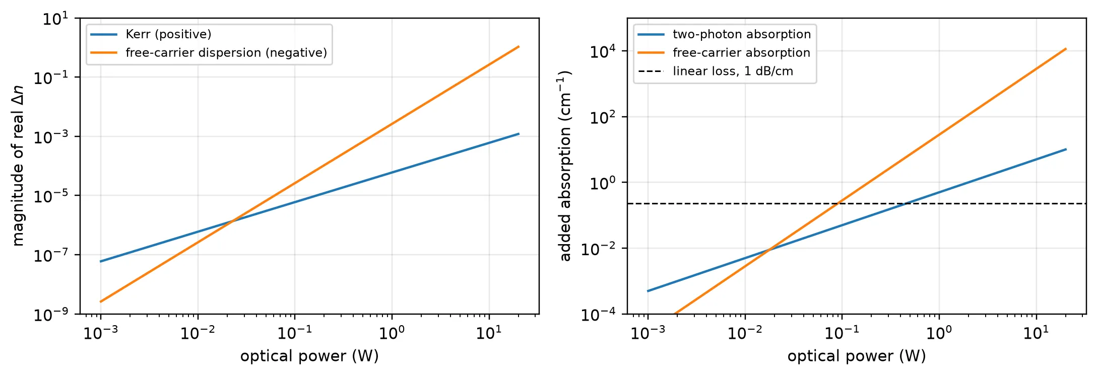

steady-state FCA exceeds TPA above 18 mW

The Kerr and TPA terms grow linearly with power, the free-carrier terms quadratically, so the free carriers are negligible at low power and dominate at high power. The two real parts have opposite signs: the Kerr effect raises the index while the free carriers lower it, so their chirps oppose each other.

The crossing power is a steady-state figure. It applies to signals much longer than the 1 ns carrier lifetime. A pulse of duration $T \ll \tau_c$ ends before the carriers approach $N_\mathrm{ss}$: they accumulate to only about $T/\tau_c$ of it, so for picosecond pulses the free carriers matter only at watt-level peak powers.

Self-phase modulation with two-photon absorption

A Gaussian pulse enters the waveguide, with envelope $A(0,t) = \sqrt{P_0}\,e^{-t^2/2T_0^2}$ and $T_0$ = 10 ps, the half-width at 1/e of the peak power. The Kerr effect turns the power profile of the pulse into a phase profile, which chirps the pulse and broadens its spectrum.

Choosing the peak power. SPM spectra are usually labelled by the maximum nonlinear phase $\phi_\mathrm{max}$, reached at the pulse peak. Without TPA, the peak intensity decays as $I_0 e^{-\alpha z}$ along the waveguide, and the Kerr phase accumulates as

$$\phi_\mathrm{max} = \int_0^L k_0\, n_2\, I_0\, e^{-\alpha z}\,\mathrm{d}z = k_0\, n_2\, I_0\, L_\mathrm{eff} = \gamma P_0 L_\mathrm{eff}.$$

The peak power that gives a chosen phase is therefore $P_0 = \phi_\mathrm{max}/(\gamma L_\mathrm{eff})$. This phase is only a label for the input power: TPA removes power along the way, so the phase actually accumulated is smaller. The same $P_0$ is passed as peak_power, so the stepper chooses its sections for this pulse.

Closed-form solution. With free carriers neglected, Yin and Agrawal give the output intensity and nonlinear phase at each instant of the pulse:

$$I(L,t) = \frac{I(0,t)\,e^{-\alpha L}}{1+\beta_\mathrm{TPA} I(0,t) L_\mathrm{eff}}, \qquad \phi(L,t) = \frac{k_0 n_2}{\beta_\mathrm{TPA}} \ln\!\left[1+\beta_\mathrm{TPA} I(0,t) L_\mathrm{eff}\right].$$

The logarithm is the central result. The nonlinear phase grows ever more slowly with input intensity, so more power in a silicon wire buys less and less additional broadening. The closed-form values at the pulse peak are printed next to the simulated ones.

Time grid. A time step of 0.1 ps gives 100 samples per half-width and a simulated bandwidth of 10 THz, far wider than the broadened spectrum. The record of 6000 steps (600 ps) holds the pulse and the 280 ps group delay of the waveguide, $n_g L/c$.

Reading the spectrum. The stepper removes the carrier, so a component of the envelope that rotates as $e^{+i2\pi\nu t}$ lies at the optical frequency $f_c - \nu$. The spectrum function uses this to place the Fourier transform of the envelope on a wavelength axis.

# Set the time grid
time_step = 1e-13  # Time step: 0.1 ps (s)
n_samples = 6000  # Record length: 600 ps
peak_step = 500  # Time step of the input pulse peak: 50 ps into the record
t = (np.arange(n_samples) - peak_step) * time_step

# Set the input pulse half-width at 1/e of the peak power (s)
t0 = 10e-12

# Set the plotted wavelength range and the power threshold for the phase
window = 1.5  # Half-width of the plotted wavelength range (nm)
threshold = 1e-3  # Fraction of the peak power above which the phase is measured

def spectrum(field):
    """Power spectral density of an envelope against wavelength (nm)."""
    # Take the power spectrum of the envelope, centred on the carrier
    psd = np.abs(np.fft.fftshift(np.fft.fft(field))) ** 2

    # Compute the frequency offset of each spectral sample from the carrier (Hz)
    nu = np.fft.fftshift(np.fft.fftfreq(field.size, time_step))

    # Convert each offset to a wavelength, the offset nu lying at f_c - nu
    return 1e9 * C_0 * 1e-6 / (carrier_frequency - nu), psd

# Create one panel per nonlinear phase
fig, axes = plt.subplots(1, 2, figsize=(10, 3.5), tight_layout=True)
for ax, phi_max in zip(axes, [1.5 * np.pi, 7.5 * np.pi]):
    # Set the peak power that gives this phase without TPA
    peak_power = phi_max / (gamma * l_eff)
    peak_intensity = peak_power / area

    # Create the Gaussian pulse envelope, in square root of watts
    pulse = np.sqrt(peak_power) * np.exp(-0.5 * (t / t0) ** 2) + 0j

    # Propagate through the wire with the Kerr effect and TPA
    out = propagate(silicon_wire(peak_power=peak_power), pulse, time_step)

    # Plot the output spectrum around the carrier wavelength
    lam_nm, psd = spectrum(out)
    keep = np.abs(lam_nm - wavelength * 1e3) < window
    ax.plot(lam_nm[keep], psd[keep] / psd[keep].max(), lw=1.4)
    ax.set_xlabel("wavelength (nm)")
    ax.set_ylabel("normalised spectral density")
    ax.set_title(
        rf"$\phi_\mathrm{{max}}$ = {phi_max / np.pi:.1f}$\pi$, "
        rf"$I_0$ = {peak_intensity / 1e13:.1f} GW/cm$^2$",
        fontsize=9.5,
    )

    # Measure the nonlinear phase as the phase swing across the pulse
    power = np.abs(out) ** 2
    phase = np.unwrap(np.angle(out))[power > threshold * power.max()]

    # Compute the closed-form peak intensity and phase at the output
    closed_intensity = (
        peak_intensity
        * np.exp(-alpha * length * 1e-6)
        / (1 + tpa * peak_intensity * l_eff)
    )
    closed_phase = k0 * kerr_index / tpa * np.log1p(tpa * peak_intensity * l_eff)

    # Print the simulated values next to the closed-form ones (GW/cm^2 and pi)
    print(
        f"phi_max = {phi_max / np.pi:.1f} pi: "
        f"output peak intensity {power.max() / area / 1e13:.3f} "
        f"(closed form {closed_intensity / 1e13:.3f}), "
        f"nonlinear phase {np.ptp(phase) / np.pi:.2f} pi "
        f"(closed form {closed_phase / np.pi:.2f} pi)"
    )
plt.show()

phi_max = 1.5 pi: output peak intensity 0.387 (closed form 0.387), nonlinear phase 1.05 pi (closed form 1.05 pi)
phi_max = 7.5 pi: output peak intensity 0.653 (closed form 0.653), nonlinear phase 2.73 pi (closed form 2.73 pi)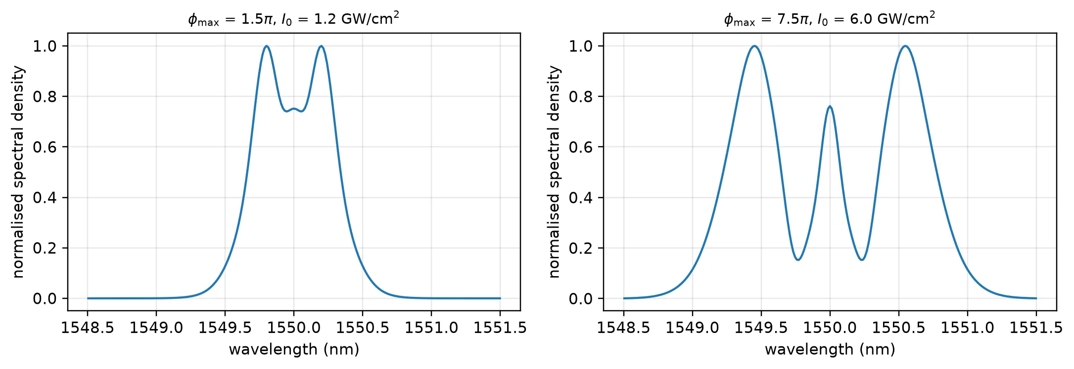

The spectrum develops the multiple peaks that are the signature of self-phase modulation, with the outermost pair the strongest. Raising $\phi_\mathrm{max}$ from 1.5π to 7.5π, a fivefold increase in power, adds peaks but broadens the spectrum far less than fivefold: TPA limits the accumulated phase to 2.73π instead of 7.5π, the saturation that the logarithm describes. The simulated phase and output intensity are those of the closed form, because the stepper has cut the wire finely enough for each pulse. How finely is the subject of the next subsection.

How many sections

A single section applies the whole nonlinear phase at once, computed from the input power. The real waveguide applies it continuously, while loss and TPA lower the power along the way. The lumped version is accurate only while the phase and the power change per section are small, so the number of sections needed grows with the nonlinear phase. With peak_power set, the stepper takes

$$N = \left\lceil \frac{k_0 L\,\lvert \Delta n_\mathrm{K}(P_0) \rvert}{\phi_\mathrm{step}} \right\rceil,$$

the Kerr phase over the whole length at the peak power, including the TPA term, divided by max_phase $\phi_\mathrm{step}$. The cell below sends the 7.5π pulse through 1 to 64 sections set explicitly with sections, and through the automatic count, and measures the nonlinear phase.

# Set the pulse that gives 7.5 pi of phase without TPA
phi_max = 7.5 * np.pi
peak_power = phi_max / (gamma * l_eff)
pulse = np.sqrt(peak_power) * np.exp(-0.5 * (t / t0) ** 2) + 0j

# Compute the closed-form nonlinear phase at the pulse peak
peak_intensity = peak_power / area
closed_phase = k0 * kerr_index / tpa * np.log1p(tpa * peak_intensity * l_eff)

def nonlinear_phase(waveguide):
    """Phase swing across the output pulse, in units of pi."""
    # Propagate the pulse and keep the samples that carry significant power
    out = propagate(waveguide, pulse, time_step)
    power = np.abs(out) ** 2
    return np.ptp(np.unwrap(np.angle(out))[power > threshold * power.max()]) / np.pi

# Propagate through waveguides cut into more and more sections
counts = [1, 2, 4, 8, 16, 32, 64]
phases = [nonlinear_phase(silicon_wire(sections=count)) for count in counts]

# Compute the automatic section count and propagate with it
automatic = int(np.ceil(k0 * length * 1e-6 * abs(tables["dn_kerr"](peak_power)) / 0.05))
automatic_phase = nonlinear_phase(silicon_wire(peak_power=peak_power))

# Plot the nonlinear phase against the number of sections
fig, ax = plt.subplots(figsize=(5.6, 3.3), tight_layout=True)
ax.semilogx(counts, phases, "o-", ms=5, label="sections set explicitly")
ax.semilogx(automatic, automatic_phase, "s", ms=7, label="automatic, from peak_power")
ax.axhline(closed_phase / np.pi, color="k", ls="--", lw=1, label="closed form")
ax.set_xlabel("number of sections")
ax.set_ylabel(r"nonlinear phase ($\pi$)")
ax.legend(fontsize=8)
plt.show()

# Print the phase for each count and for the automatic one
for count, phase in zip(counts, phases):
    print(f"{count:4d} sections: {phase:.3f} pi")
print(
    f"{automatic:4d} sections (automatic): {automatic_phase:.3f} pi, "
    f"closed form {closed_phase / np.pi:.3f} pi"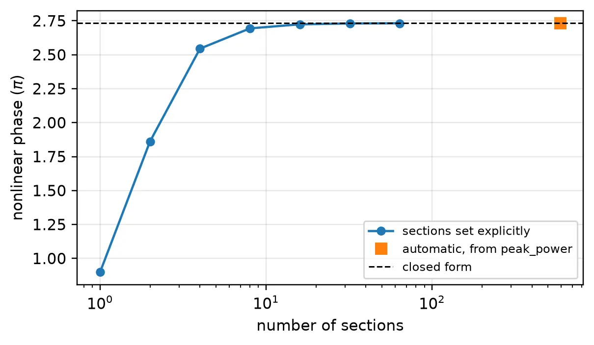
)

   1 sections: 0.899 pi
   2 sections: 1.862 pi
   4 sections: 2.545 pi
   8 sections: 2.694 pi
  16 sections: 2.724 pi
  32 sections: 2.730 pi
  64 sections: 2.732 pi
 592 sections (automatic): 2.732 pi, closed form 2.733 pi

With one section the phase is 9.36π, which is $k_0 n_2 I_0 L$: the input power applied over the whole length, with neither the linear loss nor TPA reducing it. As the section count grows, the phase approaches the closed-form 2.73π, and the remaining difference roughly halves each time the count doubles, the behaviour of a first-order split-step scheme. For this pulse the automatic count is 592 sections, which leaves 0.002π between the phase and the closed form. max_phase therefore sets the accuracy, and the number of sections follows from the pulse.

Free carriers

Two-photon absorption leaves electron-hole pairs behind, and in silicon they live for about a nanosecond, fifty times longer than the 20 ps pulse. Their density therefore keeps rising through the whole pulse instead of following its power, which is what dn_fc reproduces with tau_fc set to the carrier lifetime.

The consequence is an asymmetry in time. The leading edge of the pulse meets almost no carriers, while the trailing edge travels through all the carriers the leading edge created.

The pulse is now set for $\phi_\mathrm{max} = 15.5\pi$, a peak intensity of 12.5 GW/cm², where the free carriers are strong. Three runs add the effects one at a time: TPA alone, then FCA, then FCD with the linear coefficient $\sigma_n = -1.35\times10^{-27}$ m³ used by Yin and Agrawal.

# Set the pulse that gives 15.5 pi of phase without TPA
phi_max = 15.5 * np.pi
peak_power = phi_max / (gamma * l_eff)
pulse = np.sqrt(peak_power) * np.exp(-0.5 * (t / t0) ** 2) + 0j
print(
    f"peak intensity {peak_power / area / 1e13:.1f} GW/cm^2, "
    f"carrier lifetime {carrier_lifetime * 1e9:.0f} ns, "
    f"pulse width {2 * t0 * 1e12:.0f} ps"
)

# Switch the free-carrier effects on one at a time
cases = {
    "TPA only": dict(carriers=False),
    "TPA + FCA": dict(carriers=True, fcd_on=False),
    "TPA + FCA + FCD": dict(carriers=True, fcd_on=True),
}
outputs = {
    label: propagate(silicon_wire(peak_power=peak_power, **options), pulse, time_step)
    for label, options in cases.items()
}

# Set the plot ranges around the output pulse (ps) and the carrier wavelength (nm)
time_window = 30
spectral_window = 5

# Locate the output pulse peak without free carriers, the time origin of the plot
peak_index = int(np.argmax(np.abs(outputs["TPA only"]) ** 2))

# Create panels for the pulse shape and the spectrum
fig, axes = plt.subplots(1, 2, figsize=(10, 3.6), tight_layout=True)
for label, out in outputs.items():
    # Plot the output power against time
    axes[0].plot(
        (t - t[peak_index]) * 1e12, np.abs(out) ** 2 * 1e3, lw=1.4, label=label
    )

    # Plot the output spectrum around the carrier wavelength
    lam_nm, psd = spectrum(out)
    keep = np.abs(lam_nm - wavelength * 1e3) < spectral_window
    axes[1].plot(lam_nm[keep], psd[keep] / psd[keep].max(), lw=1.3, label=label)

# Label both panels
axes[0].set_xlabel("time (ps)")
axes[0].set_ylabel("output power (mW)")
axes[0].set_xlim(-time_window, time_window)
axes[0].set_title("pulse shape", fontsize=9.5)
axes[1].set_xlabel("wavelength (nm)")
axes[1].set_ylabel("normalised spectral density")
axes[1].set_title("spectrum", fontsize=9.5)
for ax in axes:
    ax.legend(fontsize=8)
plt.show()

# Print the energy left in each half of the pulse (pJ)
for label in ("TPA only", "TPA + FCA"):
    power = np.abs(outputs[label]) ** 2
    leading = power[:peak_index].sum() * time_step * 1e12
    trailing = power[peak_index:].sum() * time_step * 1e12
    print(
        f"{label:9s}: leading half {leading:6.3f} pJ, trailing half {trailing:6.3f} pJ"
    )

peak intensity 12.5 GW/cm^2, carrier lifetime 1 ns, pulse width 20 ps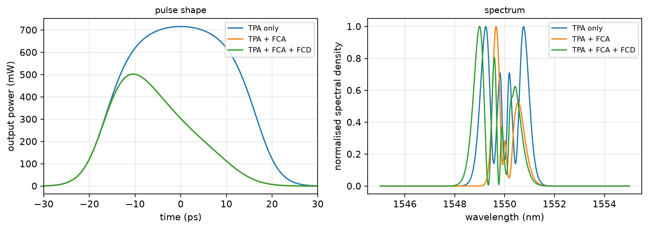

TPA only : leading half 11.050 pJ, trailing half 11.121 pJ
TPA + FCA: leading half  8.018 pJ, trailing half  2.543 pJ

Free-carrier absorption removes most of the trailing half of the pulse, leaving 2.5 pJ of 11.1 pJ, while the leading half keeps 8.0 of 11.0 pJ, and the output peak moves 10 ps earlier. Self-phase modulation puts the red-shifted light on the leading edge and the blue-shifted light on the trailing edge, so cutting the trailing edge cuts the blue side of the spectrum: the peak near 1549.2 nm disappears and the spectrum becomes lopsided rather than simply weaker.

Free-carrier dispersion acts in the other direction. Its index change is negative and grows during the pulse, which shifts light towards shorter wavelengths: the spectrum moves to the blue and gains a peak near 1549.0 nm. FCD changes only the phase, so in the pulse-shape panel its curve lies on top of the FCA one. The free carriers therefore cannot be treated as an extra loss: they change where the light ends up in the spectrum, not only how much of it survives.

The section count still comes from the Kerr phase alone, 1222 sections here. With free carriers this strong it holds the output energy within 0.3% of a run with four times as many sections.

Chromatic dispersion

Chromatic dispersion makes the group velocity depend on frequency. It is described by the group-velocity dispersion $\beta_2 = \mathrm{d}^2\beta/\mathrm{d}\omega^2$, the second derivative of the propagation constant, and acts over the dispersion length $L_D = T_0^2/\lvert \beta_2 \rvert$. For the 10 ps pulse above and $\beta_2$ = 1 ps²/m, $L_D$ is 100 m, so dispersion is negligible in a 2 cm waveguide. For a pulse with $T_0$ = 100 fs, $L_D$ falls to 1 cm, and dispersion and the nonlinear phase act over the same distance.

The class method takes the dispersion in the same form as the frequency-domain model, as the dispersion parameter $D$ in s/µm² rather than as $\beta_2$. The two are related by

$$D = -\frac{2\pi c}{\lambda^2}\,\beta_2 .$$

The stepper applies the dispersion as a finite impulse response filter on the envelope, one per section, which interleaves it with the nonlinear phase.

With anomalous dispersion ($\beta_2 < 0$), the dispersive chirp and the Kerr chirp have opposite signs. For a pulse $A(0,t) = \sqrt{P_0}\,\mathrm{sech}(t/T_0)$ they cancel exactly when the soliton order

$$N^2 = \frac{\gamma P_0 T_0^2}{\lvert \beta_2 \rvert}$$

equals one, and the pulse propagates without changing shape. This is a fundamental soliton, with peak power $P_0 = \lvert \beta_2 \rvert/(\gamma T_0^2)$. Three runs over one dispersion length compare dispersion alone, the soliton without any loss, and the soliton with the TPA and linear loss of silicon.

The time step is reduced to 10 fs, giving 10 samples per half-width, and the record of 200 ps holds the 140 ps group delay of the 1 cm waveguide.

# Set the anomalous group-velocity dispersion and the short pulse width
beta2 = -1e-24  # Group-velocity dispersion beta_2: -1 ps^2/m (s^2/m)
t0_short = 100e-15  # Pulse half-width T0 (s)

# Convert beta_2 to s^2/um, then to the dispersion parameter D (s/um^2)
dispersion = -2 * np.pi * C_0 * (beta2 * 1e-6) / wavelength**2

# Compute the peak power of the fundamental soliton, N = 1 (W)
soliton_power = abs(beta2) / (gamma * t0_short**2)

# Set the waveguide length to one dispersion length (um)
dispersion_length = t0_short**2 / abs(beta2) * 1e6
print(
    f"D = {dispersion:.3e} s/um^2, "
    f"dispersion length {dispersion_length * 1e-3:.1f} mm, "
    f"soliton peak power {soliton_power * 1e3:.0f} mW"
)

# Set the finer time grid
step_short = 1e-14  # Time step: 10 fs (s)
n_short = 20000  # Record length: 200 ps
peak_short = 3000  # Time step of the input pulse peak: 30 ps into the record
plot_range = 700  # Half-width of the plotted time range (fs)
t_short = (np.arange(n_short) - peak_short) * step_short

# Create the sech pulse, clipping the argument so cosh does not overflow in the wings
sech = np.sqrt(soliton_power) / np.cosh(np.clip(t_short / t0_short, -300, 300)) + 0j

# Switch the Kerr effect and the losses on or off for each run
runs = {
    "dispersion only": dict(kerr=False, tpa_on=False, linear_loss=False),
    "soliton, lossless": dict(kerr=True, tpa_on=False, linear_loss=False),
    "soliton in silicon": dict(kerr=True, tpa_on=True, linear_loss=True),
}

# Plot the input pulse, centred on its peak (fs)
fig, ax = plt.subplots(figsize=(6.4, 3.6), tight_layout=True)
power_in = np.abs(sech) ** 2
ax.plot(
    (t_short - t_short[peak_short]) * 1e15,
    power_in / power_in.max(),
    "k",
    lw=2,
    label="input",
)

for label, options in runs.items():
    # Propagate through one dispersion length of dispersive waveguide
    waveguide = silicon_wire(
        peak_power=soliton_power,
        dispersion=dispersion,
        total_length=dispersion_length,
        **options,
    )
    out = propagate(waveguide, sech, step_short)

    # Plot the output pulse, centred on its own peak
    power = np.abs(out) ** 2
    shift = t_short[int(np.argmax(power))]
    ax.plot((t_short - shift) * 1e15, power / power.max(), lw=1.4, label=label)

    # Measure the full width at half maximum of the output pulse (fs)
    above = power > power.max() / 2
    width = (t_short[above][-1] - t_short[above][0]) * 1e15
    print(
        f"{label:18s}: output width {width:4.0f} fs, "
        f"peak power {power.max() * 1e3:5.1f} mW"
    )

# Label the plot
ax.set_xlabel("time (fs)")
ax.set_ylabel("normalised power")
ax.set_xlim(-plot_range, plot_range)
ax.legend(fontsize=8)
ax.set_title("one dispersion length of propagation", fontsize=9.5)
plt.show()

# Print the input full width at half maximum, 1.763 T0 for a sech pulse
print(f"input width {1.763 * t0_short * 1e15:.0f} fs")

D = 7.840e-16 s/um^2, dispersion length 10.0 mm, soliton peak power 411 mW
dispersion only   : output width  260 fs, peak power 293.0 mW
soliton, lossless : output width  170 fs, peak power 410.7 mW
soliton in silicon: output width  190 fs, peak power 267.8 mW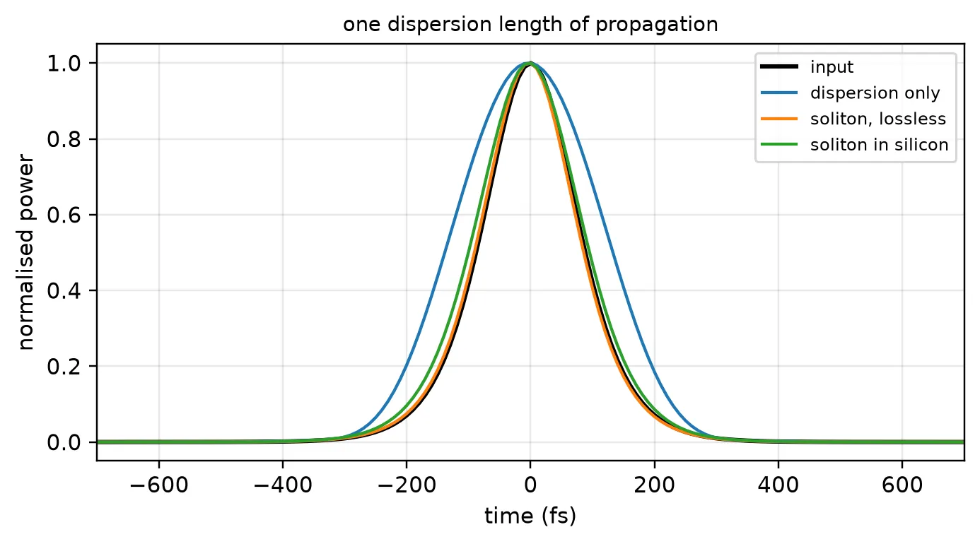

input width 176 fs

Dispersion alone stretches the pulse from 176 fs to 260 fs, by about half again, over one dispersion length. With the matched Kerr phase the lossless pulse keeps its width and peak power, since the nonlinear chirp cancels the dispersive one. In silicon the width is still close to the input, but TPA and the 1 dB/cm linear loss have taken a third of the peak power. The balance depends on that power, so over longer distances the pulse broadens. Soliton propagation over many dispersion lengths is therefore a result for silicon nitride, which has no TPA at 1550 nm, rather than for silicon.

A routed spiral from its cross-section

A real device is a routed waveguide, here a rectangular spiral of 2 cm drawn in the basic technology. The same class method applies, with two differences:

• the material coefficients live on the Tidy3D medium of the silicon core, as a nonlinear_spec with a KerrNonlinearity and a TwoPhotonAbsorption. Tidy3D states them in µm-based units: $n_2$ in µm²/W, $\beta_\mathrm{TPA}$ in µm/W, $\sigma_a$ in µm², and the plasma-dispersion coefficients $c_e, c_h$ in µm$^{3e}$. The same medium can be used in a nonlinear FDTD simulation. The values below are those of silicon at 1550 nm, with the Soref and Bennett form of free-carrier dispersion, $e_h = 0.8$;
• the cross-section is given by its port specification, "Strip". The class method runs one mode solve at the carrier frequency and takes $n_\mathrm{eff}$, $n_g$, $D$ and the effective areas from it, reading the nonlinear coefficients from the core medium. The values it used are stored in the properties of the returned model.

No length is given: the model is added to the spiral, and the stepper measures the length of the routed path from the layout.

# Describe the nonlinearity of silicon at 1550 nm on its Tidy3D medium
silicon_nonlinearity = td.NonlinearSpec(
    models=[
        td.KerrNonlinearity(n2=6e-6),  # n2: 6e-18 m^2/W (um^2/W)
        td.TwoPhotonAbsorption(
            beta=5e-6,  # beta_TPA: 5e-12 m/W (um/W)
            tau=1e-9,  # Carrier lifetime (s)
            sigma=1.45e-9,  # FCA cross section: 1.45e-21 m^2 (um^2)
            c_e=-8.8e-10,  # Soref electron term: -8.8e-22 cm^3 (um^3)
            c_h=-3.38e-8,  # Soref hole term: -8.5e-18 cm^2.4 (um^2.4)
            e_h=0.8,  # Soref hole exponent
        ),
    ]
)
silicon = td.Medium(
    permittivity=3.476**2, nonlinear_spec=silicon_nonlinearity, name="Si"
)

# Create the technology with the nonlinear silicon core
technology = pf.basic_technology(core_medium=silicon)

# Draw a 2 cm rectangular spiral with the strip cross-section
spiral = pf.parametric.rectangular_spiral(
    port_spec="Strip",
    full_length=length,
    radius=10.0,  # Bend radius (um)
    technology=technology,
)
viewer(spiral)

LayoutSchematic

The model is created from the port specification, with the peak power of the 7.5π pulse of the silicon wire, and added to the spiral as its active model. Explicit arguments take precedence over the medium, so a second model with the linear free-carrier dispersion of the silicon wire, $\sigma_n = -1.35\times10^{-27}$ m³, differs from the first only in that term. The mode solve runs once: the second call reuses its result.

# Set the peak power of the 7.5 pi pulse of the silicon wire (W)
peak_power = 7.5 * np.pi / (gamma * l_eff)

# Create the model from the strip cross-section, with every coefficient from the medium
soref_model = pf.AnalyticWaveguideModel.nonlinear(
    reference_frequency=carrier_frequency,
    port_spec="Strip",
    technology=technology,
    propagation_loss=loss,
    peak_power=peak_power,
    verbose=False,
)

# Create a second model that replaces the Soref terms with the linear coefficient
linear_model = pf.AnalyticWaveguideModel.nonlinear(
    reference_frequency=carrier_frequency,
    port_spec="Strip",
    technology=technology,
    propagation_loss=loss,
    fcd_coefficients=(fcd, 0.0),
    fcd_exponents=(1.0, 1.0),
    peak_power=peak_power,
    verbose=False,
)

# Print the cross-section parameters the mode solve supplied
properties = soref_model.properties
print(f"n_eff = {properties.n_eff:.4f}, n_group = {properties.n_group:.3f}")
print(f"D = {properties.dispersion / 1e-18:.0f} ps/(nm km)")
print(f"Kerr effective area = {properties.kerr_effective_area * 1e12:.4f} um^2")
print(f"TPA effective area = {properties.tpa_effective_area * 1e12:.4f} um^2")
print(f"routed length = {pf.route_length(spiral) * 1e-4:.4f} cm")

n_eff = 2.4400, n_group = 4.046
D = 1446 ps/(nm km)
Kerr effective area = 0.0909 um^2
TPA effective area = 0.0909 um^2
routed length = 2.0000 cm

The same pulse is sent through the silicon wire of the first part, whose parameters are those of Yin and Agrawal, and through the spiral with each of the two models, free carriers included in all three.

# Create the input pulse at this peak power
pulse = np.sqrt(peak_power) * np.exp(-0.5 * (t / t0) ** 2) + 0j

# Propagate through the silicon wire with free carriers
outputs = {
    "silicon wire, Yin and Agrawal": propagate(
        silicon_wire(peak_power=peak_power, carriers=True), pulse, time_step
    )
}

# Propagate through the spiral with each model active in turn
for label, model in (
    ("spiral, linear FCD", linear_model),
    ("spiral, Soref FCD", soref_model),
):
    spiral.add_model(model, label, set_active=True)
    outputs[label] = propagate(spiral, pulse, time_step)

# Plot the output spectra over a wider range, since the Soref terms shift further
wide_window = 3.0  # Half-width of the plotted wavelength range (nm)
fig, ax = plt.subplots(figsize=(6.4, 3.4), tight_layout=True)
for label, out in outputs.items():
    lam_nm, psd = spectrum(out)
    keep = np.abs(lam_nm - wavelength * 1e3) < wide_window
    ax.plot(lam_nm[keep], psd[keep] / psd[keep].max(), lw=1.4, label=label)

# Label the plot
ax.set_xlabel("wavelength (nm)")
ax.set_ylabel("normalised spectral density")
ax.legend(fontsize=8)
plt.show()

# Print the output peak power, energy and mean wavelength of each case
for label, out in outputs.items():
    power = np.abs(out) ** 2
    energy = power.sum() * time_step * 1e12
    lam_nm, psd = spectrum(out)
    mean_wavelength = np.sum(lam_nm * psd) / np.sum(psd)
    print(
        f"{label:30s}: peak {power.max():.3f} W, energy {energy:.2f} pJ, "
        f"mean wavelength {mean_wavelength:.3f} nm"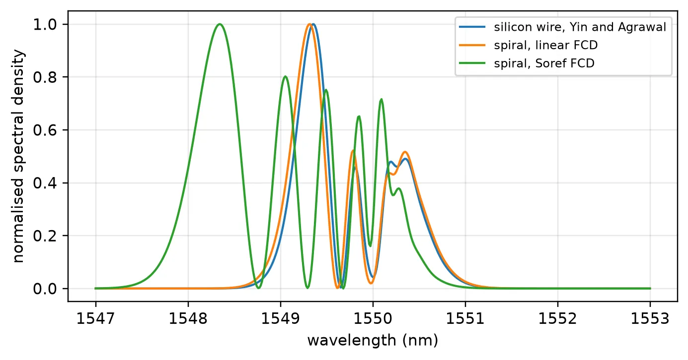
    )

silicon wire, Yin and Agrawal : peak 0.477 W, energy 10.50 pJ, mean wavelength 1549.732 nm
spiral, linear FCD            : peak 0.439 W, energy 9.59 pJ, mean wavelength 1549.714 nm
spiral, Soref FCD             : peak 0.440 W, energy 9.59 pJ, mean wavelength 1548.998 nm

With the same linear free-carrier dispersion, the spiral and the silicon wire give nearly the same spectrum: their mean wavelengths differ by 0.02 nm. The effective area from the mode solve, 0.091 µm², is 9% smaller than the 0.1 µm² of Yin and Agrawal, so the same power is a higher intensity, and the extra TPA and free-carrier absorption leave 9.56 pJ at the output instead of 10.47 pJ.

The Soref and Bennett form moves the spectrum a further 0.72 nm to the blue and adds a peak near 1548.3 nm. The pulse creates up to about 10¹⁸ cm⁻³ carriers near the input, and at 10¹⁷ to 10¹⁸ cm⁻³ the hole term $c_h N^{0.8}$ makes the index change two to three times what the linear coefficient gives. The output energy is the same in both cases, since free-carrier dispersion only changes the phase.

Summary

• pf.AnalyticWaveguideModel.nonlinear builds a waveguide model with its nonlinear time stepper from physical parameters: the Kerr and TPA coefficients, the free-carrier coefficients and lifetime, and the cross-section. The same model goes on an abstract black box or on a routed layout, whose length the stepper measures.
• Given a port specification, it takes $n_\mathrm{eff}$, $n_g$, $D$ and the effective areas from a mode solve, and the nonlinear coefficients from the nonlinear_spec of the core’s Tidy3D medium. The effective area uses the vectorial definition normalised by the mode power.
• In the stepper, the Kerr effect and TPA go on dn_kerr, and the free carriers on dn_fc with tau_fc equal to the carrier lifetime. For a free-carrier index that is not proportional to the density, dn_fc_map relaxes the density and converts it afterwards.
• The stepper splits the waveguide into sections, a split-step scheme. Passing peak_power chooses their number so that the Kerr phase per section stays below max_phase.
• Two-photon absorption makes the nonlinear phase grow only logarithmically with input power. Free carriers add an asymmetry in time and, through the chirp, an asymmetry in the spectrum.
• Set dispersion when the dispersion length is comparable to the waveguide length. For a picosecond pulse in a centimetre of silicon it is not; for a femtosecond pulse it is.