Polarizing Beam Splitter

Download notebook (.zip)

In this notebook, we reproduce the main simulation and design results presented in [1].

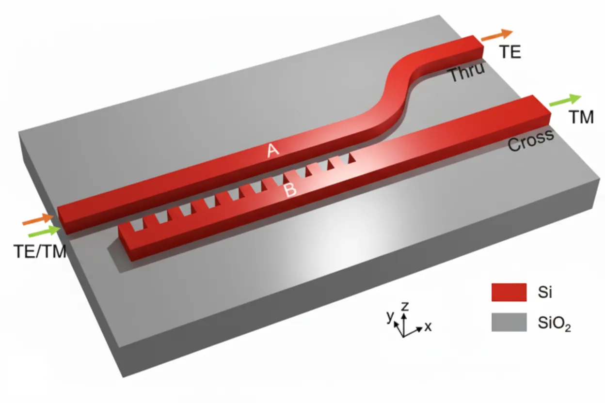
The paper introduces a polarizing beam splitter (PBS) implemented on a silicon-on-insulator (SOI) platform. The device is based on an asymmetric directional coupler (ADC) composed of a conventional strip waveguide and a subwavelength grating (SWG) waveguide. By engineering the SWG geometry, the design achieves phase matching for TM polarization while maintaining a compact footprint and broadband operation.

In this notebook, we follow a systematic workflow to reproduce and analyze the results of the SWG-assisted PBS:

1. Technology setup: define the SOI platform, wavelength range, and mesh parameters.
2. Port definition and mode analysis: construct and visualize the optical modes for both strip and SWG waveguides to ensure proper confinement and polarization behavior.
3. Component construction: build the asymmetric directional coupler geometry with user-defined SWG parameters (period, duty cycle, and gap).
4. Frequency-domain simulation: compute the scattering matrix ($S$-parameters) to extract transmission spectra for TE and TM inputs.
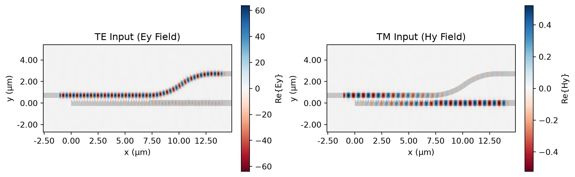
5. Field visualization: plot the electric and magnetic field distributions to confirm polarization-selective coupling.

This structured approach reproduces the key experimental and simulated trends reported in the paper while maintaining flexibility for parameter exploration and design optimization.

References

1. Zhang, Fang, et al. “Ultra-broadband and compact polarizing beam splitter in silicon photonics.” OSA Continuum 2020 3 (3), 560-567, doi: 10.1364/OSAC.385546.

import matplotlib.pyplot as plt
import numpy as np
import photonforge as pf
import siepic_forge as siepic
import tidy3d as td
from photonforge.live_viewer import LiveViewer

viewer = LiveViewer()

LiveViewer started at http://127.0.0.1:44321. Call its 'stop()' method to free the port.

Technology and Simulation Setup

We begin by defining the SiEPIC EBeam technology in PhotonForge. This technology provides a realistic silicon-on-insulator (SOI) process definition used in experimental photonic platforms. The top oxide is removed (include_top_opening=True) to match the air-clad structure used in the paper.

# Initialize the EBeam technology with top oxide removed (air cladding)
tech = siepic.ebeam(top_oxide_thickness=0.0)

# Set default technology for PhotonForge simulations
pf.config.default_technology = tech

# Define wavelength sweep range
wavelengths = np.linspace(1.45, 1.65, 51)
freqs = pf.C_0 / wavelengths

Defining Port Specifications

We next define the input/output port specifications for both the regular strip and SWG waveguides.

• The strip waveguide has a width of 0.48 µm, matching the standard single-mode silicon waveguide used in the paper.
• The SWG-equivalent waveguide has a slightly larger effective width of 0.555 µm, consistent with the optimized design parameters that achieve TM phase matching.
• Both ports support two optical modes, enabling simulation of both TE and TM fundamental modes.
• The path_profiles parameter defines the waveguide cross-section profile used by PhotonForge to construct the port geometry.

# Define the width of the regular silicon strip waveguide (µm)
w_strip = 0.48

# Define the width of the subwavelength grating (SWG) equivalent waveguide (µm)
w_swg = 0.555

# Create a port specification for the strip waveguide
port_spec_strip = pf.PortSpec(
    description="Multi mode strip",  # descriptive label for identification
    width=2.5,  # total port width (simulation window)
    num_modes=2,  # number of supported optical modes
    target_neff=3.5,  # target effective index for solver initialization
    limits=(-1.5, 1.22),  # vertical boundaries of the simulation domain
    path_profiles=[
        (w_strip, 0, (1, 0))
    ],  # waveguide path geometry (width, offset, direction)
)

# Create a port specification for the SWG (subwavelength) waveguide
port_spec_swg = pf.PortSpec(
    description="Multi mode swg",
    width=2.5,
    num_modes=2,
    target_neff=3.5,
    limits=(-1.5, 1.22),
    path_profiles=[(w_swg, 0, (1, 0))],
)

Before proceeding to coupling simulations, it is essential to inspect the mode field profiles of each port.
We visually verify that the fields are well confined within the waveguide core and decay to near-zero amplitude at the port boundaries.

# Compute modes for both ports at 1.55 µm (f = c / λ)
f0 = pf.C_0 / 1.55

# Strip port modes
mode_solver_strip = pf.port_modes(port_spec_strip, [f0], mesh_refinement=30)

# SWG port modes
mode_solver_swg = pf.port_modes(port_spec_swg, [f0], mesh_refinement=30)

# Create a 2×2 figure layout for two modes (m=0,1) of both ports
fig, axes = plt.subplots(2, 2, figsize=(10, 8), constrained_layout=True)

mode_solver_strip.plot_field("E", mode_index=0, f=f0, ax=axes[0, 0])
mode_solver_strip.plot_field("H", mode_index=1, f=f0, ax=axes[0, 1])
mode_solver_swg.plot_field("E", mode_index=0, f=f0, ax=axes[1, 0])
mode_solver_swg.plot_field("H", mode_index=1, f=f0, ax=axes[1, 1])
axes[0, 0].set_title("Strip | TE Mode")
axes[0, 1].set_title("Strip | TM Mode")
axes[1, 0].set_title("SWG | TE Mode")
axes[1, 1].set_title("SWG | TM Mode")
# Add a shared figure title
fig.suptitle("Port Mode Fields at λ = 1.55 µm", y=1.02)
plt.show()

Uploading task 'Mode-ModeSolver…'
Starting task 'Mode-ModeSolver': https://tidy3d.simulation.cloud/workbench?taskId=mo-35e5df16-b4ce-4e3a-99fa-da320c14c547
Downloading data from 'Mode-ModeSolver'…
Uploading task 'Mode-ModeSolver…'
Starting task 'Mode-ModeSolver': https://tidy3d.simulation.cloud/workbench?taskId=mo-1f1e0325-9984-489c-821f-8b45bcf17b40
Downloading data from 'Mode-ModeSolver'…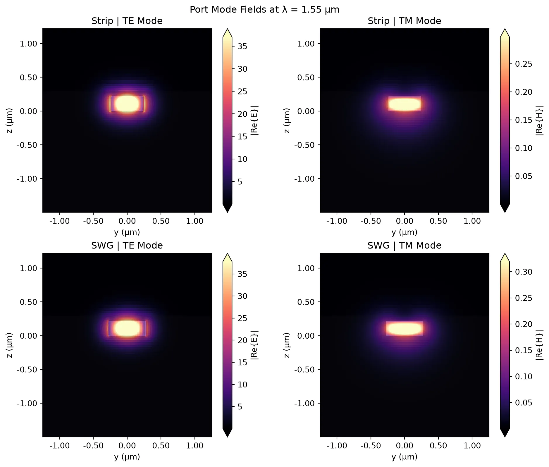

Creating PBS

We define a parametric component that constructs the SWG-assisted asymmetric coupler used as a polarizing beam splitter:

• The SWG region is generated by repeating a unit cell with period $\Lambda$ and duty cycle $f$, producing a coupling length $L_c = N\Lambda$.
• The strip waveguide is routed to run parallel through the coupling region and then transitions via an S-bend to separate the outputs.
• Ports are detected and added using the provided PortSpecs, allowing us to excite and monitor TE/TM modes consistently across runs.
• A Tidy3D model is attached for subsequent FDTD simulations using the same geometric object.

# Define a parametric component for the SWG-assisted PBS
@pf.parametric_component
def create_pbs(
    *,
    spec_strip=port_spec_strip,
    spec_swg=port_spec_swg,
    w_corrugation=0.130,
    gap=0.200,
    swg_period=0.240,
    swg_duty_cycle=0.5,
    n_periods=30,
    s_bend_length=6,
    s_bend_offset=2,
):
    # Resolve string-based specs from the default technology if needed
    if isinstance(spec_strip, str):
        spec_strip = pf.config.default_technology.ports[spec_strip]
    if isinstance(spec_swg, str):
        spec_swg = pf.config.default_technology.ports[spec_swg]

    # Extract effective silicon widths from the provided PortSpecs
    w_strip, _ = spec_strip.path_profile_for("Si")
    w_swg, _ = spec_swg.path_profile_for("Si")

    # Compute total coupling length from SWG period and number of periods
    coupling_length = n_periods * swg_period

    # Create one SWG unit cell component consisting of ridge + groove
    unit_cell = pf.Component("SWG Period")

    # Build the ridge and groove rectangles for one period
    ridge_length = swg_duty_cycle * swg_period
    ridge = pf.Rectangle((0, -w_swg / 2), (ridge_length, w_swg / 2))
    groove = pf.Rectangle(
        (ridge_length, -w_swg / 2), (swg_period, w_swg / 2 - w_corrugation)
    )

    # Add ridge and groove into the unit cell along +x
    unit_cell.add((1, 0), ridge, groove)

    # Create the parent PBS component
    pbs = pf.Component("PBS")

    # Instantiate the SWG array by repeating the unit cell N times
    swg_array = pf.Reference(
        component=unit_cell, columns=n_periods, rows=1, spacing=(swg_period, 0.0)
    )

    # Add a short straight continuation for the SWG waveguide after coupling region
    swg_wg = pf.Rectangle(
        (coupling_length, -w_swg / 2),
        (coupling_length + s_bend_length + 0.1, w_swg / 2),
    )

    # Route the strip waveguide: lead-in, straight through coupler, then S-bend
    strip_wg = (
        pf.Path(origin=(-1.0, gap + (w_swg + w_strip) / 2), width=w_strip)
        .segment(endpoint=(coupling_length + 1.0, 0), relative=True)
        .s_bend(endpoint=(s_bend_length, s_bend_offset), relative=True)
    )

    # Add geometry to the PBS component (placed along +x)
    pbs.add((1, 0), swg_array, strip_wg, swg_wg)

    # Detect and add ports for strip (input) and SWG (output on +x boundary)
    pbs.add_port(pbs.detect_ports([spec_strip]))
    pbs.add_port(pbs.detect_ports([spec_swg], on_boundary="+x"))

    # Attach a Tidy3D model for simulation
    pbs.add_model(
        pf.Tidy3DModel(
            monitors=[
                td.FieldMonitor(
                    name="field",
                    center=(0, 0, 0.11),
                    size=(td.inf, td.inf, 0),
                    freqs=[pf.C_0 / 1.55],
                )
            ],
        )
    )
    return pbs

# Instantiate and view the PBS component with default parameters
pbs = create_pbs()
viewer(pbs)

LayoutSchematic

Transmission for TM and TE Inputs

We compute $S$-parameters over the wavelength sweep and plot transmission in dB as $10\log_{10}|S|^2$:

• The left panel shows TM input with cross and thru responses, including a small inset emphasizing the cross band.
• The right panel shows TE input with cross and thru responses.

s_matrix = pbs.s_matrix(freqs, model_kwargs={"inputs": ["P0"]})

Uploading task 'P0@0…'
Uploading task 'P0@1…'
Starting task 'P0@0': https://tidy3d.simulation.cloud/workbench?taskId=fdve-1ce4e54d-dc0a-48ac-a14d-49a7e60b0ace
Starting task 'P0@1': https://tidy3d.simulation.cloud/workbench?taskId=fdve-fedbe98a-fe3c-4476-8115-44bbca7f302b
Downloading data from 'P0@0'…
Downloading data from 'P0@1'…

# Define key mapping for S-parameters
k_te_thru = ("P0@0", "P1@0")  # TE input → through
k_te_cross = ("P0@0", "P2@0")  # TE input → cross
k_tm_thru = ("P0@1", "P1@1")  # TM input → through
k_tm_cross = ("P0@1", "P2@1")  # TM input → cross

# Helper to convert complex S-parameter to transmission in dB
def s_to_db(s):
    """
    Return 10*log10(|S|^2) with small floor for numerical stability.
    """
    return 10.0 * np.log10(np.abs(s) ** 2 + 1e-18)

# Extract wavelength axis in nm
wl_nm = wavelengths * 1e3

# Create side-by-side plots for TM input and TE input
fig, axes = plt.subplots(1, 2, figsize=(10, 4), constrained_layout=True)

# TM input: plot cross and thru
ax_tm = axes[0]
ax_tm.plot(wl_nm, s_to_db(s_matrix[k_tm_cross]), label="cross", linewidth=2)
ax_tm.plot(wl_nm, s_to_db(s_matrix[k_tm_thru]), label="thru", linewidth=2)
ax_tm.set_xlabel("Wavelength (nm)")
ax_tm.set_ylabel("Transmission (dB)")
ax_tm.set_title("TM input")
ax_tm.legend(loc="center", frameon=False)

# Optional inset for TM cross near 1450–1650 nm
from mpl_toolkits.axes_grid1.inset_locator import inset_axes

axins = inset_axes(ax_tm, width="30%", height="30%", loc="lower left", borderpad=2)
axins.plot(wl_nm, s_to_db(s_matrix[k_tm_cross]), linewidth=1.5)
axins.set_xticks([1450, 1550, 1650])
axins.set_yticks([-2, -1, 0])
axins.set_title("cross", fontsize=9, pad=2)

# TE input: plot cross and thru
ax_te = axes[1]
ax_te.plot(wl_nm, s_to_db(s_matrix[k_te_cross]), label="cross", linewidth=2)
ax_te.plot(wl_nm, s_to_db(s_matrix[k_te_thru]), label="thru", linewidth=2)
ax_te.set_xlabel("Wavelength (nm)")
ax_te.set_ylabel("Transmission (dB)")
ax_te.set_title("TE input")
ax_te.legend(loc="center", frameon=False)

# Add an overall style tweak
for ax in axes.ravel():
    ax.grid(True, alpha=0.2)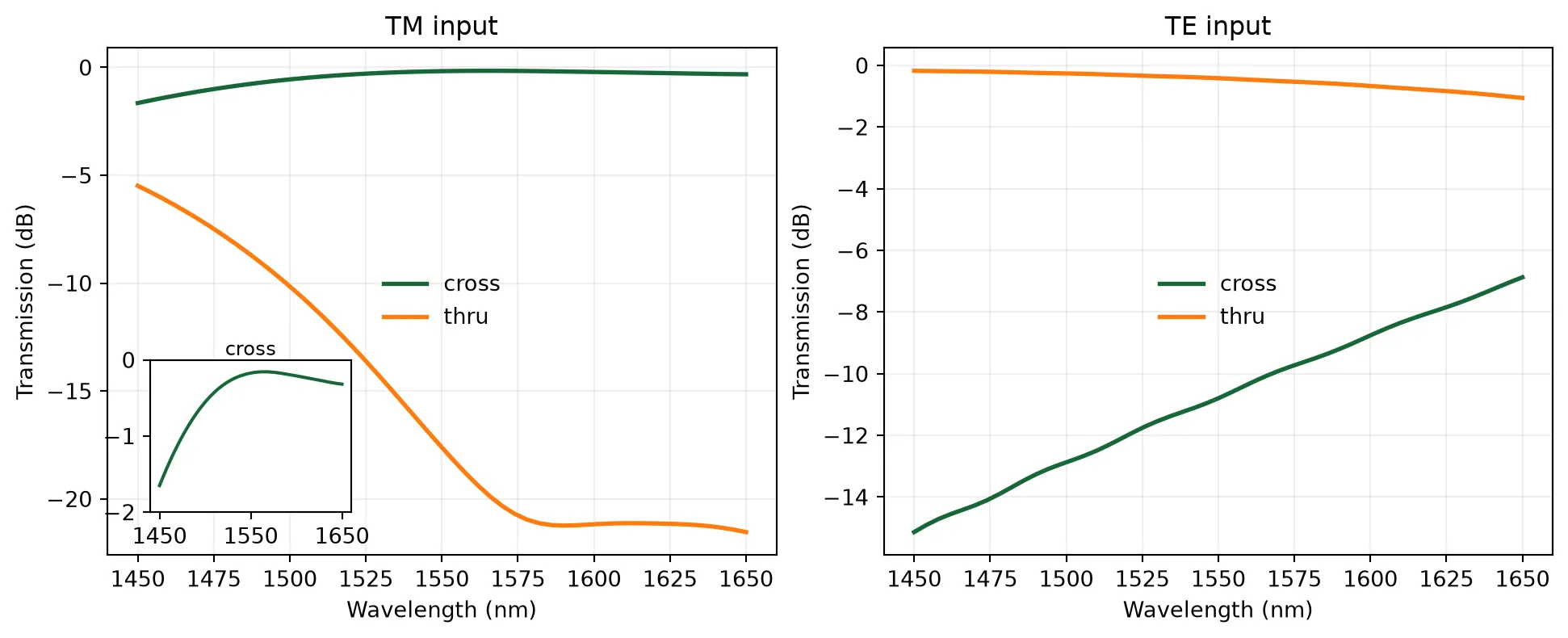

Finally, we visualize the simulated field distributions of the polarizing beam splitter.

# Retrieve simulation field data for PBS model
sim_data_pbs = pbs.active_model.batch_data(pbs, freqs, inputs=["P0"])

# Create a 1×2 subplot figure
fig, axes = plt.subplots(1, 2, figsize=(10, 3), constrained_layout=True)

# Plot Ey field for TE input (P0@0)
ax0 = sim_data_pbs["P0@0"].plot_field("field", "Ey", ax=axes[0], robust=False)
axes[0].set_title("TE Input (Ey Field)")

# Plot Hy field for TM input (P0@1)
ax1 = sim_data_pbs["P0@1"].plot_field("field", "Hy", ax=axes[1], robust=False)
axes[1].set_title("TM Input (Hy Field)")
plt.show()

14:29:53 -03 Loading simulation from local cache. View cached task using web UI 
             at                                                                 
             'https://tidy3d.simulation.cloud/workbench?taskId=fdve-1ce4e54d-dc0
             a-48ac-a14d-49a7e60b0ace'.                                         

             Loading simulation from local cache. View cached task using web UI 
             at                                                                 
             'https://tidy3d.simulation.cloud/workbench?taskId=fdve-fedbe98a-fe3
             c-4476-8115-44bbca7f302b'.