Electro-Absorption Modulator

Download notebook (.zip)

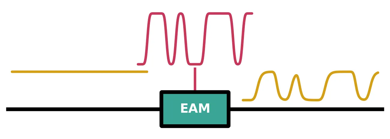
An electro-absorption modulator (EAM) is a short waveguide section made of a semiconductor whose absorption edge lies just below the photon energy of the light. A reverse bias across a p-i-n junction puts an electric field on the absorbing core, and the field moves the absorption edge to longer wavelengths. The light is absorbed more strongly as the reverse bias grows, so the transmitted power follows the drive voltage directly. In bulk semiconductors such as germanium the mechanism is the Franz-Keldysh effect [2]; in quantum wells it is the quantum-confined Stark effect. Germanium EAMs on silicon are only tens of micrometres long, have junction capacitances of a few femtofarads, and need no traveling-wave electrode, which makes them compact, fast and efficient intensity modulators for short-reach links [1, 3].

ElectroAbsorptionModTimeStepper models the modulator in the time domain: the bias-dependent absorption, a bias-independent insertion loss, the chirp of the modulated light, the RC low-pass of the junction, and the photocurrent generated by the absorbed light. The absorption is supplied as a table over voltage and wavelength, which franz_keldysh_absorption can generate for a bulk absorber. electro_absorption_modulator wraps it in a component with two optical ports, P0 and P1, and one electrical port, E0. The same component also carries an AnalyticWaveguideModel with the same table for frequency-domain simulations at a fixed bias.

This guide shows how to use them for a germanium EAM on silicon, with the device parameters of Liu et al. [1]: building and calibrating the absorption table, the transmission spectra, the transfer curve against bias, the photocurrent, the modulation bandwidth, the eye diagram of non-return-to-zero (NRZ) data, and the chirp.

References

1. Liu, Y., Sun, J., Song, R., et al. “80Gb/s NRZ Ge waveguide electro-absorption modulator.” Optics Express 2022 30 (19), 34276-34286, doi: 10.1364/OE.462890.
2. Chuang, S. L. Physics of Photonic Devices, 2nd ed. Wiley 2009.
3. Liu, J., Beals, M., Pomerene, A., et al. “Waveguide-integrated, ultralow-energy GeSi electro-absorption modulators.” Nature Photonics 2008 2 (7), 433-437, doi: 10.1038/nphoton.2008.99.
4. Koyama, F., and Iga, K. “Frequency chirping in external modulators.” Journal of Lightwave Technology 1988 6 (1), 87-93, doi: 10.1109/50.3969.

What the time stepper computes

Let $\alpha(V, \lambda)$ be the absorption coefficient of the material at the applied voltage $V$ and the wavelength $\lambda$. Only the fraction $\Gamma$ of the optical mode that overlaps the absorbing core is absorbed, so the power decays along the section as $\mathrm{d}P/\mathrm{d}z = -\Gamma\alpha P$. Over the length $\ell$ the power transmission is $e^{-\Gamma\alpha\ell}$, and the field is multiplied by the square root of this factor.

A change of absorption always comes with a change of refractive index, so the phase of the light follows its intensity. The chirp parameter $\alpha_c$ of the modulator, as defined by Koyama and Iga [4] and quoted on datasheets, relates the instantaneous frequency deviation of the output to its power:

$$\delta\nu = \frac{\alpha_c}{4\pi}\,\frac{\mathrm{d}\ln P}{\mathrm{d}t}.$$

PhotonForge uses the $e^{-j\omega t}$ time convention, in which an envelope $e^{-j 2\pi \Delta f\, t}$ is light at $f_0 + \Delta f$, so the frequency deviation is $\delta\nu = -(1/2\pi)\,\mathrm{d}\phi/\mathrm{d}t$ for an envelope phase $\phi$. The chirp therefore appears as the phase $+\alpha_c\Gamma\alpha\ell/2$, and with a bias-independent loss $L_0$ in dB the output field is

$$A_\mathrm{out} = A_\mathrm{in}\,10^{-L_0/20}\,\exp\!\left[-\frac{\Gamma\alpha(V)\ell}{2} \left(1 - j\alpha_c\right)\right],$$

with $P = \lvert A \rvert^2$. The absorption table is evaluated once, at the carrier wavelength, because the absorption edge varies over terahertz while a data signal occupies tens of gigahertz.

The voltage $V$ is the sum of a constant bias and the drive read from the electrical port. A signal of amplitude $A_\mathrm{e}$ on that port becomes a voltage through the port impedance $Z_0$, $V_\mathrm{drive} = \Re\{A_\mathrm{e}\}\sqrt{Z_0}$. Before it reaches the absorber, the drive passes through a first-order low-pass with the cutoff $f_\mathrm{3dB}$, which represents the charging of the junction capacitance $C_j$ through the series resistance $R_s$, $f_\mathrm{3dB} = 1/(2\pi R_s C_j)$.

Every absorbed photon can generate an electron-hole pair, which the junction field collects. With the quantum efficiency $\eta$, the photon energy $h\nu$ and the elementary charge $q$, the photocurrent is

$$I_\mathrm{ph} = \eta\,\frac{q}{h\nu}\,P_\mathrm{in}\left(1 - e^{-\Gamma\alpha(V)\ell}\right),$$

and it is emitted on the electrical port as the amplitude $-I_\mathrm{ph}\sqrt{Z_0}$.

The component’s parameters map onto these quantities as follows:

• absorption is the table $\alpha(V, \lambda)$ in 1/μm, as an Interpolator over voltage and wavelength.
• length is $\ell$ in μm, and confinement_factor is $\Gamma$.
• bias is the constant bias in V. Reverse bias is negative.
• residual_loss is $L_0$ in dB, for example the loss of the transitions into and out of the absorbing section.
• chirp is $\alpha_c$.
• f_3dB is the cutoff of the junction low-pass in Hz. None disables the filter.
• quantum_efficiency is $\eta$. A value of 0 disables the photocurrent.
• n_group is the group index for the optical transit delay through the section. The default, 0, disables the delay.

Setup

The device of Liu et al. [1] is a germanium waveguide 600 nm wide, 350 nm tall and 40 μm long, grown in a recess of a 220 nm silicon-on-insulator waveguide, with a lateral p-i-n junction across the germanium. The measured values used below are:

• Insertion loss at 1603 nm: 5.73 dB, of which 1.06 dB is the loss of the two transitions between the silicon and the germanium waveguides.
• Static extinction ratio between 0 V and -3 V at 1603 nm: 14.15 dB.
• Series resistance 250 Ω and junction capacitance 4.8 fF, from a fit to the measured electrical reflection.
• Responsivity as a photodetector at -3 V and 1610 nm: 1.04 A/W.
• Drive for the eye diagrams: 2.3 V peak to peak around a -3 V bias.

The confinement factor is not reported. A mode solve of the germanium core in its silicon recess places 85% of the mode intensity in the germanium, and we use $\Gamma = 0.85$.

import matplotlib.pyplot as plt
import numpy as np
import photonforge as pf
import photonforge.abstract as pfa

# Open the live viewer to display the modulator component
viewer = pf.live_viewer.LiveViewer()

# Use the basic technology for the abstract components
pf.config.default_technology = pf.basic_technology()

# Set the physical constants for the photon energy and the photocurrent
h_planck = 6.62607015e-34  # Planck constant (J s)
q = 1.602176634e-19  # Elementary charge (C)

# Set the operating wavelength and the carrier frequency (pf.C_0 is in um/s)
wavelength = 1.603  # Operating wavelength (um)
f0 = pf.C_0 / wavelength  # Carrier frequency (Hz)

# Set the geometry and the measured losses of the modulator
length = 40.0  # Length of the germanium section (um)
confinement = 0.85  # Confinement factor of the mode in the germanium
insertion_loss = 5.73  # Measured insertion loss at 0 V (dB)
transition_loss = 1.06  # Loss of the two silicon-germanium transitions (dB)

# Set the electrical parameters of the junction
r_s = 250.0  # Series resistance (Ohm)
c_j = 4.8e-15  # Junction capacitance (F)
z0 = 50.0  # Reference impedance of the electrical port (Ohm)

# Set the operating point of the drive
bias = -3.0  # Reverse bias of the junction (V)
v_pp = 2.3  # Peak-to-peak drive voltage (V)

# Compute the RC cutoff of the junction, 1 / (2 pi R_s C_j)
f_rc = 1 / (2 * np.pi * r_s * c_j)
print(f"RC cutoff frequency: {f_rc / 1e9:.1f} GHz")

LiveViewer started at http://127.0.0.1:42949. Call its 'stop()' method to free the port.
RC cutoff frequency: 132.6 GHz

Absorption table from the Franz-Keldysh effect

The electric field $F$ across the intrinsic region tilts the bands of the semiconductor. An electron can then absorb a photon with an energy below the bandgap and tunnel the rest of the way into the conduction band. The absorption edge acquires a tail below the bandgap that grows with the field, which is the Franz-Keldysh effect. With the reduced effective mass $m_r$ of the electron and the light hole, the field sets the energy scale

$$\hbar\theta = \left(\frac{q^2\hbar^2F^2}{2m_r}\right)^{1/3},$$

and the absorption at the photon energy $\hbar\omega$ below the bandgap energy $E_g$ is [2]

$$\alpha(\hbar\omega, F) = \alpha_s\,\frac{\sqrt{\hbar\theta}}{\hbar\omega} \left[\mathrm{Ai}'(\beta)^2 - \beta\,\mathrm{Ai}(\beta)^2\right], \qquad \beta = \frac{E_g - \hbar\omega}{\hbar\theta},$$

where $\mathrm{Ai}$ is the Airy function and $\alpha_s$ a scale constant. The field follows from the voltage across the intrinsic width $d$ and the built-in potential $V_{bi}$ of the junction, $F = (V_{bi} - V)/d$, so a negative (reverse) bias increases the field.

pf.franz_keldysh_absorption evaluates this expression on a grid of wavelengths and voltages and returns the table as an interpolator. Only the dependence on photon energy and field is physical; the absolute scale $\alpha_s$, the absorption_scale argument, is calibrated to one measured value. We calibrate it to the measured insertion loss at 0 V. Without the transitions, the germanium section loses $5.73 - 1.06 = 4.67$ dB, and a loss $L$ in dB corresponds to

$$\alpha = \frac{L}{10\log_{10}(e)\,\Gamma\ell}.$$

The table uses an intrinsic width of 0.4 μm, the 600 nm germanium core less its implanted edges, and the default built-in potential of 0.7 V and reduced mass of 0.02 electron masses. The bandgap wavelength is set to 1.582 μm, which makes the table reproduce the measured static extinction ratio. It corresponds to 0.784 eV, just below the 0.80 eV direct gap of bulk germanium, since the tensile strain of growth on silicon lowers the gap.

# Set the grid of the absorption table
wavelengths = np.linspace(1.55, 1.65, 101)  # Wavelength grid (um)
voltages = np.linspace(-5.0, 0.0, 51)  # Voltage grid (V)

# Set the Franz-Keldysh parameters of the germanium junction
fk_parameters = {
    "wavelengths": wavelengths,
    "voltages": voltages,
    "bandgap_wavelength": 1.582,  # Direct bandgap wavelength (um)
    "intrinsic_thickness": 0.4,  # Width of the intrinsic region (um)
}

# Build the table with the default absorption scale of 1
absorption_raw = pf.franz_keldysh_absorption(**fk_parameters)

# Convert the measured 0 V loss of the germanium section to an absorption (1/um)
db_per_neper = 10 * np.log10(np.e)  # Loss in dB of a power decay by e
loss_0v = insertion_loss - transition_loss  # Loss of the germanium section at 0 V (dB)
alpha_0v = loss_0v / (db_per_neper * confinement * length)

# Scale the table so that it returns alpha_0v at 0 V and the operating wavelength
alpha_raw = absorption_raw(np.array([[0.0, wavelength]]))[0]
absorption = pf.franz_keldysh_absorption(
    **fk_parameters, absorption_scale=alpha_0v / alpha_raw
)

# Evaluate the calibrated table at 0 V and at the bias, at the operating wavelength
alpha_bias = absorption(np.array([[bias, wavelength]]))[0]
print(f"Absorption at 0 V: {alpha_0v * 1e4:.0f} 1/cm")
print(f"Absorption at {bias:g} V: {alpha_bias * 1e4:.0f} 1/cm")

# Compute the static extinction ratio between 0 V and the bias (dB)
extinction_static = db_per_neper * confinement * length * (alpha_bias - alpha_0v)
print(f"Static extinction ratio, 0 V to {bias:g} V: {extinction_static:.2f} dB")

# Plot the absorption spectrum at several voltages
fig, ax = plt.subplots(figsize=(7, 3.2), tight_layout=True)
for v in [0.0, -1.0, -2.0, -3.0, -4.0]:
    # Evaluate the table along the wavelength axis at this voltage
    points = np.column_stack([np.full(wavelengths.size, v), wavelengths])
    ax.semilogy(wavelengths * 1e3, absorption(points) * 1e4, label=f"{v:g} V")

# Mark the operating wavelength
ax.axvline(wavelength * 1e3, color="gray", lw=0.8)
ax.set(xlabel="Wavelength (nm)", ylabel="Absorption (1/cm)", ylim=(10, 2e4))
ax.legend()
plt.show()

Absorption at 0 V: 316 1/cm
Absorption at -3 V: 1264 1/cm
Static extinction ratio, 0 V to -3 V: 13.99 dB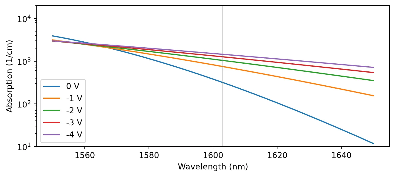

At the operating wavelength the absorption rises from 316 1/cm at 0 V to 1264 1/cm at -3 V, a factor of four, and the calibrated table gives a static extinction ratio of 13.99 dB between the two biases. The curves show how the Franz-Keldysh effect shapes the absorption:

• At wavelengths longer than the bandgap wavelength, the field raises the absorption tail. The relative change grows with wavelength, while the absorption itself falls.
• Below about 1565 nm, above the bandgap, the field lowers the absorption slightly. An EAM is therefore operated on the long-wavelength side of the edge.

Creating the modulator

pfa.electro_absorption_modulator builds the component from the table and the device parameters. The junction low-pass is set to the RC cutoff computed above, and the transitions enter as the bias-independent residual_loss.

# Create the modulator at the operating bias
eam = pfa.electro_absorption_modulator(
    absorption=absorption,
    length=length,
    confinement_factor=confinement,
    bias=bias,
    residual_loss=transition_loss,
    f_3dB=f_rc,
    z0=z0,
)
viewer(eam)

Transmission spectra

The frequency-domain model of the component evaluates the same table at the fixed bias, over any range of wavelengths. Two figures describe the static performance of an EAM at each wavelength:

• the insertion loss (IL), the loss at 0 V, including the transitions;
• the extinction ratio (ER), the ratio of the transmission at 0 V to the transmission at the reverse bias.

The next cell computes the S matrix of the component at biases from 0 V to -3 V and plots the transmission spectra, the insertion loss, and the extinction ratio at -3 V.

# Set the wavelengths of the spectra and the corresponding frequencies
spectrum_wavelengths = np.linspace(1.56, 1.64, 161)  # Wavelengths (um)
frequencies = pf.C_0 / spectrum_wavelengths  # Frequencies (Hz)

# Compute the transmission spectrum at each bias from the S matrix
transmission_db = {}
for v in [0.0, -1.0, -2.0, -3.0]:
    # Create the modulator at this bias and compute its S matrix
    component = pfa.electro_absorption_modulator(
        absorption=absorption,
        length=length,
        confinement_factor=confinement,
        bias=v,
        residual_loss=transition_loss,
    )
    s_matrix = component.s_matrix(frequencies, show_progress=False)

    # Convert the transmission from P0 to P1 to dB
    transmission_db[v] = 20 * np.log10(np.abs(s_matrix["P0@0", "P1@0"]))

# Compute the insertion loss and the extinction ratio at -3 V
il = -transmission_db[0.0]
er = transmission_db[0.0] - transmission_db[-3.0]

# Plot the transmission spectra in the left panel
fig, (ax1, ax2) = plt.subplots(1, 2, figsize=(7, 3), tight_layout=True)
for v, t_db in transmission_db.items():
    ax1.plot(spectrum_wavelengths * 1e3, t_db, label=f"{v:g} V")
ax1.set(xlabel="Wavelength (nm)", ylabel="Transmission (dB)")
ax1.legend(fontsize=7)

# Plot the insertion loss and the extinction ratio in the right panel
ax2.plot(spectrum_wavelengths * 1e3, il, label="Insertion loss")
ax2.plot(spectrum_wavelengths * 1e3, er, label="Extinction ratio at -3 V")
ax2.axvline(wavelength * 1e3, color="gray", lw=0.8)
ax2.set(xlabel="Wavelength (nm)", ylabel="Loss or ratio (dB)", ylim=(0, 30))
ax2.legend(fontsize=7)
plt.show()

# Print both figures at the operating wavelength
i_op = np.argmin(np.abs(spectrum_wavelengths - wavelength))
print(f"At {wavelength * 1e3:.0f} nm: IL {il[i_op]:.2f} dB, ER {er[i_op]:.2f} dB")

# Find the wavelength of the largest extinction ratio
i_max = np.argmax(er)
print(f"Largest ER: {er[i_max]:.2f} dB at {spectrum_wavelengths[i_max] * 1e3:.0f} nm")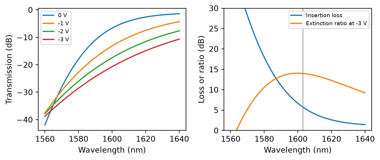

At 1603 nm: IL 5.73 dB, ER 13.99 dB
Largest ER: 14.05 dB at 1600 nm

The insertion loss falls steeply with wavelength, from 28 dB at 1570 nm to 1.4 dB at 1640 nm, where the transitions account for most of it. The extinction ratio at -3 V is largest, 14.05 dB, near 1600 nm and falls slowly on either side. The operating wavelength of 1603 nm sits at this maximum, with 5.73 dB of insertion loss. A longer wavelength trades extinction ratio for lower loss: at 1620 nm the insertion loss is 2.6 dB and the extinction ratio 12.3 dB.

Transfer curve and operating point

In the time domain the modulator is driven through its electrical port. A single component needs no surrounding circuit: setup_time_stepper returns its time stepper directly, and the inputs are passed to step as a TimeSeries keyed by port name: the optical field on "P0@0" and the drive on "E0@0". The optical fields are in √W, so $\lvert A \rvert^2$ is the power in watts, and a drive voltage $V_\mathrm{drive}$ is passed as the amplitude $V_\mathrm{drive}/\sqrt{Z_0}$.

The next cell ramps the drive slowly from -2 V to +3 V around the -3 V bias, so the applied voltage sweeps from -5 V to 0 V in a single run, and plots the transmission against the applied voltage. The ramp lasts 2 ns, far longer than the 1.2 ps time constant of the junction, so the transmission follows the static transfer curve. The dotted line is the transmission computed directly from the table, $L_0 + 10\log_{10}(e)\,\Gamma\alpha(V)\ell$ in dB of loss, for reference. The shaded band marks the 2.3 V drive swing around the bias.

The junction low-pass starts every run from 0 V, so the applied voltage takes a few time constants to reach the bias. The first 10 ps of the run are discarded for this reason.

time_step = 0.25e-12  # Simulation time step (s)
num_steps = 8000  # Number of time steps, a 2 ns ramp
p_in = 1e-3  # Input optical power (W)
settle = 40  # Time steps discarded while the junction charges to the bias

# Build the CW optical input and the slow voltage ramp of the drive
a_in = np.full(num_steps, np.sqrt(p_in), dtype=complex)  # Optical field (sqrt(W))
v_drive = np.linspace(-2.0, 3.0, num_steps)  # Drive voltage (V)

# Set up the time stepper of the modulator
time_stepper = eam.setup_time_stepper(
    time_step=time_step, carrier_frequency=f0, show_progress=False
)

# Run the ramp, passing the drive as the amplitude V / sqrt(Z0)
inputs = pf.TimeSeries({"P0@0": a_in, "E0@0": v_drive / np.sqrt(z0) + 0j}, time_step)
outputs = time_stepper.step(inputs=inputs, show_progress=False)

# Compute the transmission against the applied voltage, bias plus drive
v_applied = (bias + v_drive)[settle:]
transmission = np.abs(outputs["P1@0"][settle:]) ** 2 / p_in

# Compute the transmission from the table at the operating wavelength
points = np.column_stack([voltages, np.full(voltages.size, wavelength)])
loss_table = transition_loss + db_per_neper * confinement * length * absorption(points)

# Set the two drive levels: the one level at low reverse bias, the zero level at high
v_one = bias + v_pp / 2
v_zero = bias - v_pp / 2

# Plot the transfer curve with the drive swing
fig, ax = plt.subplots(figsize=(7, 3.2), tight_layout=True)
ax.plot(v_applied, 10 * np.log10(transmission), label="Time stepper")
ax.plot(voltages, -loss_table, "k:", label="Absorption table")
ax.axvspan(v_zero, v_one, color="gray", alpha=0.2)
ax.set(xlabel="Applied voltage (V)", ylabel="Transmission (dB)")
ax.legend()
plt.show()

# Read the transmission at the two drive levels from the ramp
t_one = np.interp(v_one, v_applied, transmission)
t_zero = np.interp(v_zero, v_applied, transmission)
print(f"Transmission at {v_one:.2f} V (one level): {10 * np.log10(t_one):.2f} dB")
print(f"Transmission at {v_zero:.2f} V (zero level): {10 * np.log10(t_zero):.2f} dB")
print(f"Dynamic extinction ratio: {10 * np.log10(t_one / t_zero):.2f} dB")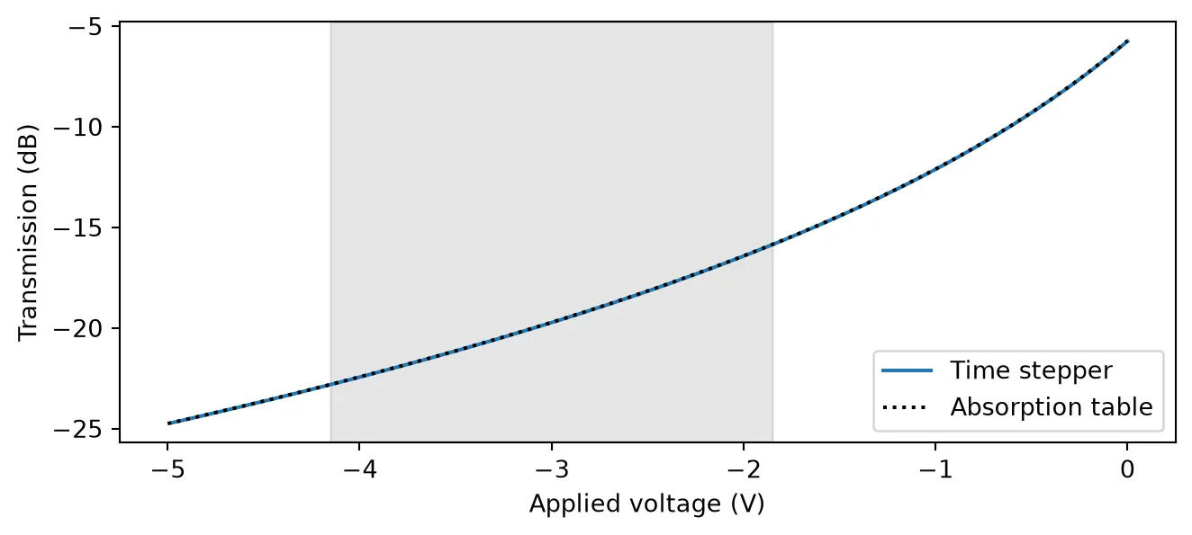

Transmission at -1.85 V (one level): -15.86 dB
Transmission at -4.15 V (zero level): -22.81 dB
Dynamic extinction ratio: 6.95 dB

The time stepper traces the same curve as the table, since at every step it evaluates the table at the applied voltage. The transmission falls from -5.73 dB at 0 V to -24.7 dB at -5 V, and the curve is steepest near 0 V. Around the -3 V bias, the 2.3 V swing gives a dynamic extinction ratio of 6.95 dB, and the one level at -1.85 V lies 15.86 dB below the input power.

The same ramp gives the two levels for any bias. The next cell moves the 2.3 V swing along the transfer curve and plots the dynamic extinction ratio and the loss of the one level against the bias.

# Sweep the bias, keeping both drive levels inside the ramp
bias_sweep = np.linspace(v_applied[0] + v_pp / 2, v_applied[-1] - v_pp / 2, 31)

# Read the transmission of both levels from the ramp (dB)
t_one_db = 10 * np.log10(np.interp(bias_sweep + v_pp / 2, v_applied, transmission))
t_zero_db = 10 * np.log10(np.interp(bias_sweep - v_pp / 2, v_applied, transmission))

# Plot the dynamic extinction ratio and the loss of the one level against the bias
fig, ax = plt.subplots(figsize=(7, 3.2), tight_layout=True)
ax.plot(bias_sweep, t_one_db - t_zero_db, label="Dynamic extinction ratio")
ax.plot(bias_sweep, -t_one_db, label="Loss of the one level")
ax.axvline(bias, color="gray", lw=0.8)
ax.set(xlabel="Bias (V)", ylabel="Loss or ratio (dB)")
ax.legend()
plt.show()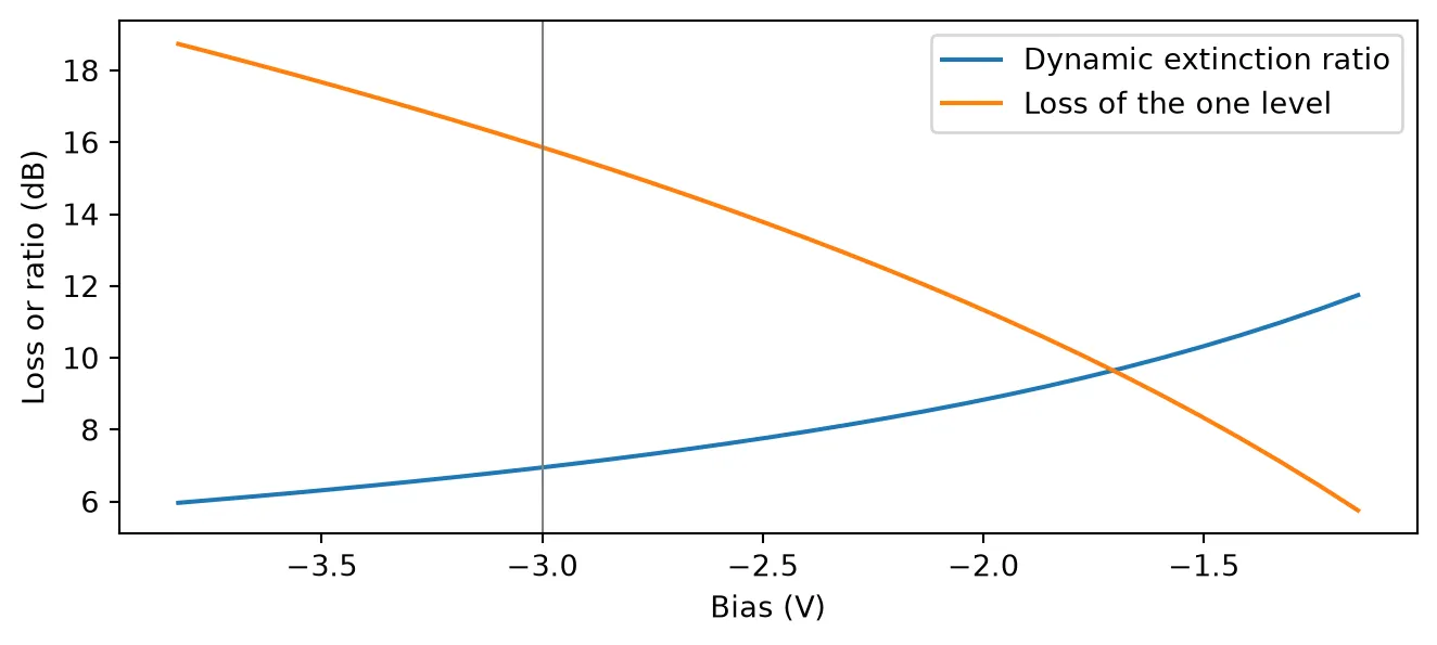

Moving the bias toward 0 V improves both figures, because the transfer curve is steepest there. At -1.15 V, where the one level reaches 0 V, the dynamic extinction ratio is 11.7 dB and the one level loses 5.8 dB, against 6.95 dB and 15.9 dB at -3 V.

Practical devices are biased deeper than this curve alone suggests. A strong field sweeps the photogenerated carriers out of the germanium quickly, which avoids absorption saturation at high optical power, and it fully depletes the intrinsic region, which keeps the junction capacitance at its minimum. Neither effect is part of the absorption table, so the bias is set from measurements of the device. The rest of this guide keeps the -3 V bias of [1].

Photocurrent

The light absorbed in the germanium is not lost: the junction collects the carriers, and the modulator also works as a photodetector. The photocurrent is emitted on the electrical port as the amplitude $-I_\mathrm{ph}\sqrt{Z_0}$, so it can load the driver in a circuit, and it can be read to monitor the optical power or the bias point.

The quantum efficiency $\eta$ is calibrated to the measured responsivity. Operated as a photodetector at -3 V and 1610 nm, the device of Liu et al. gives $R = 1.04$ A/W [1]. The responsivity of the model is $R = \eta\,(q/h\nu)\left(1 - e^{-\Gamma\alpha\ell}\right)$, so

$$\eta = \frac{R}{(q/h\nu)\left(1 - e^{-\Gamma\alpha\ell}\right)}.$$

This value of $\eta$ also absorbs the input transition, since the model refers the photocurrent to the power at the input port. The next cell computes $\eta$, recreates the modulator with it, and repeats the voltage ramp at 1 mW input power to plot the photocurrent against the applied voltage.

responsivity_measured = 1.04  # Measured responsivity at -3 V and 1610 nm (A/W)
wavelength_pd = 1.61  # Wavelength of the responsivity measurement (um)

# Compute the fraction of the light absorbed at -3 V and 1610 nm
alpha_pd = absorption(np.array([[-3.0, wavelength_pd]]))[0]
absorbed_pd = 1 - np.exp(-confinement * alpha_pd * length)

# Compute the quantum efficiency from the ideal responsivity q / (h nu)
ideal_responsivity = q / (h_planck * pf.C_0 / wavelength_pd)
eta = responsivity_measured / (ideal_responsivity * absorbed_pd)
print(f"Absorbed fraction at -3 V and 1610 nm: {absorbed_pd:.3f}")
print(f"Quantum efficiency: {eta:.3f}")

# Recreate the modulator with the calibrated quantum efficiency
eam = pfa.electro_absorption_modulator(
    absorption=absorption,
    length=length,
    confinement_factor=confinement,
    bias=bias,
    residual_loss=transition_loss,
    f_3dB=f_rc,
    quantum_efficiency=eta,
    z0=z0,
)

# Repeat the voltage ramp with the new modulator
time_stepper = eam.setup_time_stepper(
    time_step=time_step, carrier_frequency=f0, show_progress=False
)
outputs = time_stepper.step(inputs=inputs, show_progress=False)

# Convert the electrical output amplitude to the photocurrent, I = -Re(A) / sqrt(Z0)
i_ph = -outputs["E0@0"][settle:].real / np.sqrt(z0)

# Compute the responsivity at the operating wavelength from the table
responsivity_table = (
    eta * q / (h_planck * f0) * (1 - np.exp(-confinement * absorption(points) * length))
)

# Plot the photocurrent against the applied voltage
fig, ax = plt.subplots(figsize=(7, 3.2), tight_layout=True)
ax.plot(v_applied, i_ph * 1e3, label="Time stepper")
ax.plot(voltages, responsivity_table * p_in * 1e3, "k:", label="Absorption table")
ax.axvspan(v_zero, v_one, color="gray", alpha=0.2)
ax.set(xlabel="Applied voltage (V)", ylabel="Photocurrent (mA)")
ax.legend()
plt.show()

# Print the photocurrent at the two drive levels
for level, v in [("one", v_one), ("zero", v_zero)]:
    print(
        f"Photocurrent at {v:.2f} V ({level} level): "
        f"{np.interp(v, v_applied, i_ph) * 1e3:.3f} mA"
    )

Absorbed fraction at -3 V and 1610 nm: 0.978
Quantum efficiency: 0.819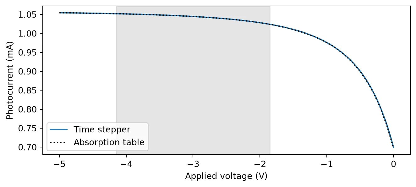

Photocurrent at -1.85 V (one level): 1.024 mA
Photocurrent at -4.15 V (zero level): 1.052 mA

The quantum efficiency comes out at 0.82: 82% of the photons absorbed in the germanium, counted at the input port, are collected as current. The rest are lost in the input transition and to recombination.

The photocurrent follows the absorbed fraction. It rises from 0.71 mA at 0 V and levels off near 1.05 mA, where almost all of the light is absorbed. Across the drive swing it changes by only 3%, from 1.024 mA at the one level to 1.052 mA at the zero level. The photocurrent flows against the bias, so with 1 mW of input power the modulator dissipates about 3.1 mW at -3 V. This heat, and the current drawn from the bias supply, grow in proportion to the optical power.

Modulation bandwidth

The Franz-Keldysh effect responds in well under a picosecond, so the speed of the modulator is set by the RC charging of the junction [1]. The time stepper applies this as a first-order low-pass on the drive, with the response

$$H(f) = \frac{1}{1 + j f/f_\mathrm{3dB}}.$$

The electro-optic (EO) response is measured the way a lightwave component analyzer measures it: a small sinusoidal drive at the frequency $f_m$ is added to the bias, and the amplitude of the resulting modulation of the output power is recorded. The next cell sweeps $f_m$ from 1 GHz to 300 GHz with a 20 mV amplitude, small enough for the transfer curve to be linear. Each run lasts 40 periods, and the amplitude is fitted over the last 20, after the filter has settled. The response is normalized to its value at the lowest frequency and shown with the RC law for reference.

v_tone = 0.02  # Amplitude of the small-signal drive (V)
num_periods = 40  # Number of drive periods in each run

# Sweep the modulation frequency (Hz)
f_mod = np.geomspace(1e9, 300e9, 25)

response = []
for f in f_mod:
    # Build the sinusoidal drive for this frequency
    t = np.arange(int(round(num_periods / f / time_step))) * time_step
    v_drive = v_tone * np.sin(2 * np.pi * f * t)

    # Run the modulator on the CW input and the drive
    time_stepper = eam.setup_time_stepper(
        time_step=time_step, carrier_frequency=f0, show_progress=False
    )
    tone_inputs = pf.TimeSeries(
        {
            "P0@0": np.full(t.size, np.sqrt(p_in), dtype=complex),
            "E0@0": v_drive / np.sqrt(z0) + 0j,
        },
        time_step,
    )
    p_out = (
        np.abs(time_stepper.step(inputs=tone_inputs, show_progress=False)["P1@0"]) ** 2
    )

    # Fit a constant plus a sinusoid at f to the second half of the output power
    half = t.size // 2
    basis = np.column_stack(
        [
            np.ones(t.size - half),
            np.cos(2 * np.pi * f * t[half:]),
            np.sin(2 * np.pi * f * t[half:]),
        ]
    )
    coefficients = np.linalg.lstsq(basis, p_out[half:], rcond=None)[0]
    response.append(np.hypot(coefficients[1], coefficients[2]))

# Normalize the response to the lowest frequency and convert to dB
response_db = 20 * np.log10(np.array(response) / response[0])

# Compute the RC law, normalized in the same way
rc_law_db = -10 * np.log10((1 + (f_mod / f_rc) ** 2) / (1 + (f_mod[0] / f_rc) ** 2))

# Plot the EO response with the RC law
fig, ax = plt.subplots(figsize=(7, 3.2), tight_layout=True)
ax.semilogx(f_mod / 1e9, response_db, "o", label="Time stepper")
ax.semilogx(f_mod / 1e9, rc_law_db, "k:", label="RC law")
ax.axhline(-3, color="gray", lw=0.8)
ax.set(xlabel="Modulation frequency (GHz)", ylabel="EO response (dB)")
ax.legend()
plt.show()

# Interpolate the frequency where the response crosses -3 dB
f_3db_eo = np.interp(3, -response_db, f_mod)
print(f"EO 3 dB bandwidth: {f_3db_eo / 1e9:.0f} GHz")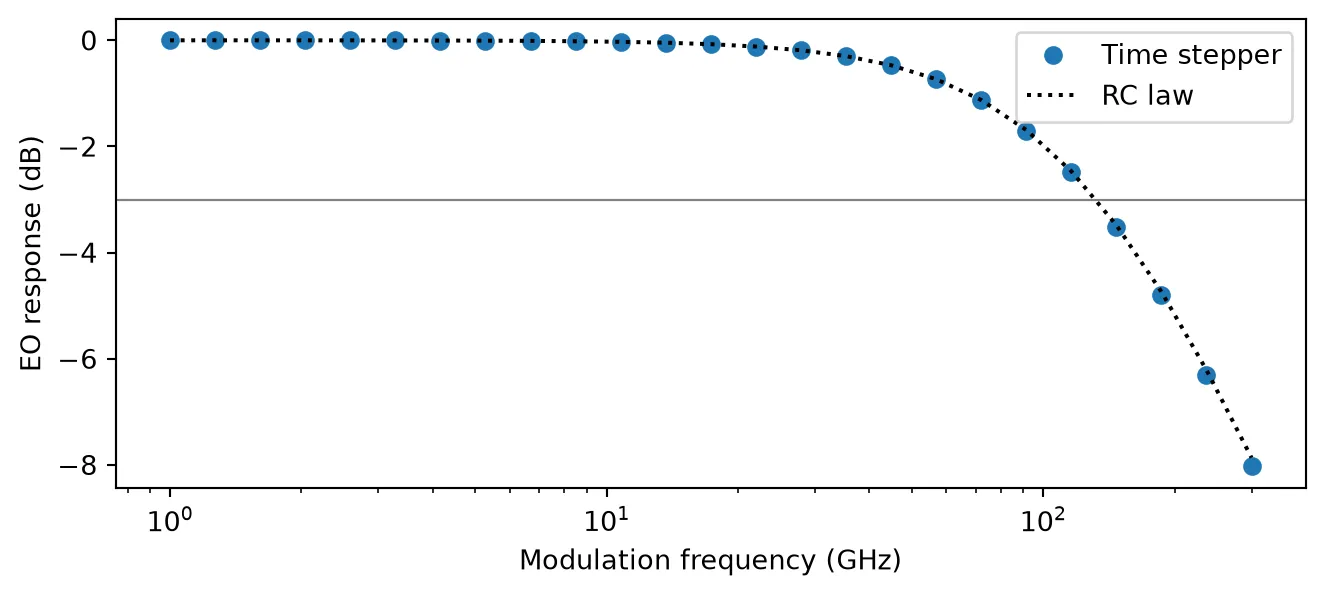

EO 3 dB bandwidth: 131 GHz

The response follows the RC law and crosses -3 dB at 131 GHz, at the RC cutoff of the junction. For comparison, [1] measured an EO bandwidth beyond 67 GHz, the upper limit of the instrument used.

Eye diagram of NRZ data

The next cell drives the modulator with random NRZ data at 2.3 V peak to peak around the -3 V bias, at 80 Gb/s, the highest rate measured in [1], and at 160 Gb/s. A one bit is the level of low reverse bias, $-3 + 1.15 = -1.85$ V, and a zero bit the level of high reverse bias, -4.15 V. The edges of the drive are smoothed with a Gaussian filter to represent the finite bandwidth of the driver. The output power is folded into two-bit segments to form the eye, and the extinction ratio is measured from the average power at the bit centers. The first two bits are discarded while the junction charges to the bias.

num_bits = 256  # Number of random bits
num_skip = 2  # Bits discarded while the junction charges to the bias
edge_fraction = 0.15  # Width of the edge-smoothing Gaussian, as a fraction of a bit

# Draw a reproducible random bit sequence
rng = np.random.default_rng(1)
bits = rng.integers(0, 2, num_bits)

fig, axes = plt.subplots(1, 2, figsize=(7, 3), sharey=True, tight_layout=True)
for ax, bit_rate in zip(axes, [80e9, 160e9]):
    # Compute the number of samples per bit, the unit interval
    unit_interval = int(round(1 / bit_rate / time_step))

    # Map the bits to drive voltages and hold each for one bit
    v_drive = np.repeat(np.where(bits == 1, v_pp / 2, -v_pp / 2), unit_interval)

    # Smooth the edges of the drive with a Gaussian filter
    width = edge_fraction * unit_interval
    k = np.arange(-4 * width, 4 * width + 1)
    kernel = np.exp(-0.5 * (k / width) ** 2)
    v_drive = np.convolve(
        np.pad(v_drive, k.size, mode="edge"), kernel / kernel.sum(), "same"
    )
    v_drive = v_drive[k.size : -k.size]

    # Run the modulator on the CW input and the data drive
    time_stepper = eam.setup_time_stepper(
        time_step=time_step, carrier_frequency=f0, show_progress=False
    )
    data_inputs = pf.TimeSeries(
        {
            "P0@0": np.full(v_drive.size, np.sqrt(p_in), dtype=complex),
            "E0@0": v_drive / np.sqrt(z0) + 0j,
        },
        time_step,
    )
    p_out = (
        np.abs(time_stepper.step(inputs=data_inputs, show_progress=False)["P1@0"]) ** 2
    )

    # Fold the output into two-bit segments, centered on the bits, to form the eye
    segments = p_out[num_skip * unit_interval + unit_interval // 2 :]
    segments = segments[: len(segments) // (2 * unit_interval) * 2 * unit_interval]
    t_eye = np.arange(2 * unit_interval) / unit_interval
    for segment in segments.reshape(-1, 2 * unit_interval):
        ax.plot(t_eye, segment * 1e6, "C0", alpha=0.15, lw=0.8)
    ax.set(title=f"{bit_rate / 1e9:g} Gb/s", xlabel="Time (bits)")

    # Measure the extinction ratio from the average power at the bit centers
    centers = p_out[np.arange(num_skip, num_bits) * unit_interval + unit_interval // 2]
    ones = centers[bits[num_skip:] == 1]
    zeros = centers[bits[num_skip:] == 0]
    ratio_db = 10 * np.log10(ones.mean() / zeros.mean())
    print(f"{bit_rate / 1e9:g} Gb/s: dynamic extinction ratio {ratio_db:.2f} dB")

axes[0].set_ylabel("Output power (µW)")
plt.show()

80 Gb/s: dynamic extinction ratio 6.83 dB
160 Gb/s: dynamic extinction ratio 6.25 dB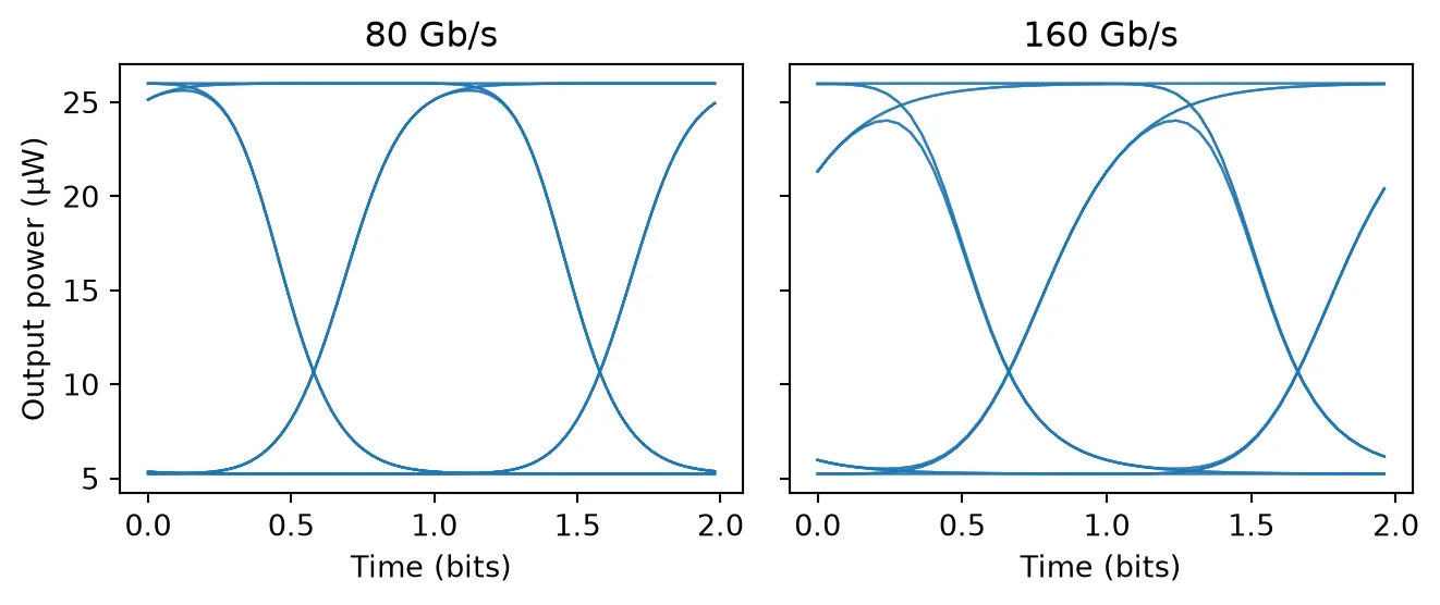

At 80 Gb/s a bit lasts 12.5 ps, ten time constants of the junction, and the eye is wide open. The dynamic extinction ratio is 6.83 dB, close to the 6.95 dB of the static levels. At 160 Gb/s a bit lasts 6.25 ps, five time constants. The junction no longer settles fully within a bit, the traces split according to the preceding bits, and the dynamic extinction ratio falls to 6.25 dB. With f_3dB=None both rates give 6.95 dB, so this closing of the eye comes from the junction RC.

Chirp

With $\alpha_c \neq 0$ the output phase follows the power, $\phi = -(\alpha_c/2)\ln P$ plus a constant. With the envelope convention above, a factor $e^{-j 2\pi \Delta f\, t}$ in $A(t)$ sits at the physical frequency $f_0 + \Delta f$, so the instantaneous frequency offset of the output is

$$\delta\nu(t) = -\frac{1}{2\pi}\frac{\mathrm{d}\phi}{\mathrm{d}t} = \frac{\alpha_c}{4\pi}\frac{\mathrm{d}\ln P}{\mathrm{d}t}.$$

The frequency moves only on the edges of the signal, where the power changes. With a positive $\alpha_c$ the rising edge shifts to higher frequencies (blue) and the falling edge to lower frequencies (red); a negative $\alpha_c$ reverses both. The sign matters in a dispersive fiber [4]. In standard single-mode fiber at 1550 nm, red light travels slower than blue, so with a negative $\alpha_c$ the red rising edge and the blue falling edge move toward the center of the pulse, and the pulse first compresses. A positive $\alpha_c$ broadens it from the start.

The chirp parameter of an EAM changes with the bias and the wavelength, because both move the operating point along the absorption edge, and it is usually taken from a measurement at the operating point. The next cell sends a single 80 Gb/s one bit through modulators with $\alpha_c = -0.5$ and $+0.5$ and plots the output power and the instantaneous frequency, with the expression above for reference.

bit_rate = 80e9  # Bit rate of the drive (b/s)

# Compute the number of samples per bit, the unit interval
unit_interval = int(round(1 / bit_rate / time_step))

# Build a single one bit between zeros, with smoothed edges
v_drive = np.repeat(
    np.where(np.array([0, 0, 1, 0, 0]) == 1, v_pp / 2, -v_pp / 2), unit_interval
)
width = edge_fraction * unit_interval
k = np.arange(-4 * width, 4 * width + 1)
kernel = np.exp(-0.5 * (k / width) ** 2)
v_drive = np.convolve(
    np.pad(v_drive, k.size, mode="edge"), kernel / kernel.sum(), "same"
)
v_drive = v_drive[k.size : -k.size]

# Set the time axis in bits, centered on the one bit
t_bits = np.arange(v_drive.size) / unit_interval - 2.5

# Select the central three bits, after the junction has charged to the bias
shown = np.abs(t_bits) < 1.5

fig, (ax1, ax2) = plt.subplots(1, 2, figsize=(7, 3), tight_layout=True)
for alpha_c in [-0.5, 0.5]:
    # Create the modulator with this chirp parameter
    chirped = pfa.electro_absorption_modulator(
        absorption=absorption,
        length=length,
        confinement_factor=confinement,
        bias=bias,
        residual_loss=transition_loss,
        f_3dB=f_rc,
        chirp=alpha_c,
        z0=z0,
    )

    # Run it on the CW input and the single-bit drive
    time_stepper = chirped.setup_time_stepper(
        time_step=time_step, carrier_frequency=f0, show_progress=False
    )
    bit_inputs = pf.TimeSeries(
        {
            "P0@0": np.full(v_drive.size, np.sqrt(p_in), dtype=complex),
            "E0@0": v_drive / np.sqrt(z0) + 0j,
        },
        time_step,
    )
    a_out = time_stepper.step(inputs=bit_inputs, show_progress=False)["P1@0"]

    # Compute the instantaneous frequency offset from the output phase (GHz)
    phase = np.unwrap(np.angle(a_out))
    delta_nu = -np.gradient(phase, time_step) / (2 * np.pi) / 1e9

    # Compute the same offset from the logarithmic derivative of the power (GHz)
    p_out = np.abs(a_out) ** 2
    delta_nu_law = alpha_c / (4 * np.pi) * np.gradient(np.log(p_out), time_step) / 1e9

    # Plot the power in the left panel and the frequency offset in the right panel
    label = f"$\\alpha_c$ = {alpha_c:g}"
    ax1.plot(t_bits[shown], p_out[shown] * 1e6, label=label)
    ax2.plot(t_bits[shown], delta_nu[shown], label=label)
    ax2.plot(t_bits[shown], delta_nu_law[shown], "k:", lw=1)

    # Find the largest frequency offset on the rising and on the falling edge (GHz)
    rising = delta_nu[shown & (t_bits < 0)]
    falling = delta_nu[shown & (t_bits > 0)]
    peak_rising = rising[np.argmax(np.abs(rising))]
    peak_falling = falling[np.argmax(np.abs(falling))]
    print(
        f"alpha_c = {alpha_c:g}: rising edge {peak_rising:.1f} GHz, "
        f"falling edge {peak_falling:.1f} GHz"
    )

# Label the power and frequency panels
ax1.set(xlabel="Time (bits)", ylabel="Output power (µW)")
ax1.legend(fontsize=7)
ax2.set(xlabel="Time (bits)", ylabel="Frequency offset (GHz)")
ax2.legend(fontsize=7)
plt.show()

alpha_c = -0.5: rising edge -11.6 GHz, falling edge 11.9 GHz
alpha_c = 0.5: rising edge 11.6 GHz, falling edge -11.9 GHz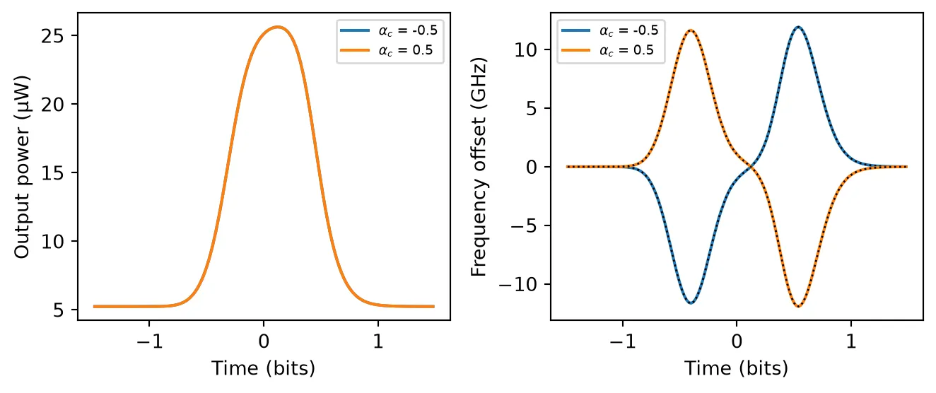

The output power is the same for both values of $\alpha_c$, since the chirp acts only on the phase. The frequency moves only on the edges, where it follows the logarithmic derivative of the power. With $\alpha_c = 0.5$ the rising edge shifts by +11.6 GHz, to the blue, and the falling edge by -11.9 GHz, to the red; $\alpha_c = -0.5$ reverses both shifts.

Summary

• pfa.electro_absorption_modulator is an EAM with two optical ports and one electrical port. It carries an AnalyticWaveguideModel for frequency-domain simulations at a fixed bias and an ElectroAbsorptionModTimeStepper for time-domain simulations driven through the electrical port.
• The absorption is a table over voltage and wavelength, sliced at the carrier wavelength. pf.franz_keldysh_absorption generates it for a bulk absorber such as germanium; its absorption_scale is calibrated to one measured loss. Quantum-well devices use a measured table instead.
• The transmission is $e^{-\Gamma\alpha(V)\ell}$ times the bias-independent residual_loss, so the transfer curve in dB follows the absorption against voltage.
• The drive voltage is $\Re\{A\}\sqrt{Z_0}$ on the electrical port, added to bias. Reverse bias is negative.
• f_3dB is the RC cutoff $1/(2\pi R_s C_j)$ of the junction and sets the modulation bandwidth.
• The absorbed light produces a photocurrent, emitted on the electrical port as $-I_\mathrm{ph}\sqrt{Z_0}$, with quantum_efficiency calibrated to a measured responsivity.
• chirp is the modulator chirp parameter $\alpha_c$ as quoted on datasheets, which shifts the frequency on the edges of the signal by $(\alpha_c/4\pi)\,\mathrm{d}\ln P/\mathrm{d}t$: a positive value blue-shifts the rising edge.