Link Simulation

Download notebook (.zip)

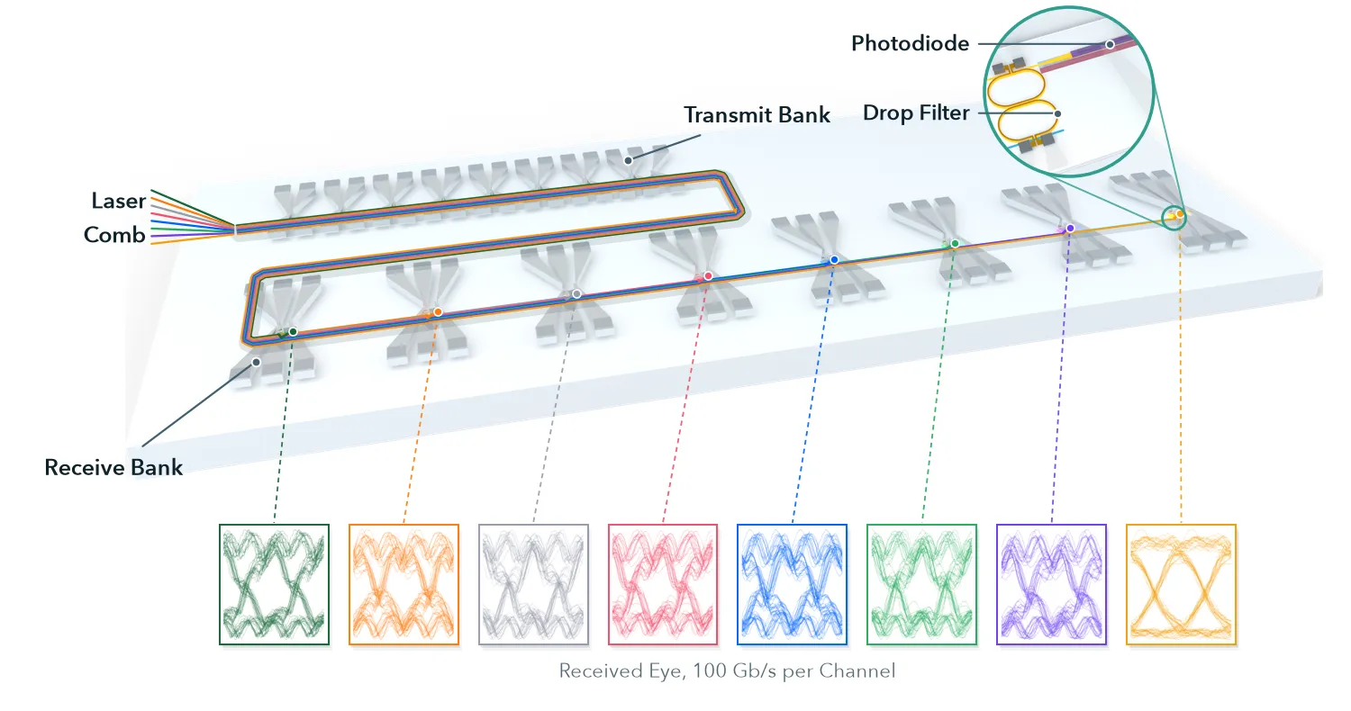
The chip the series arrives at, with the part this notebook works on marked:

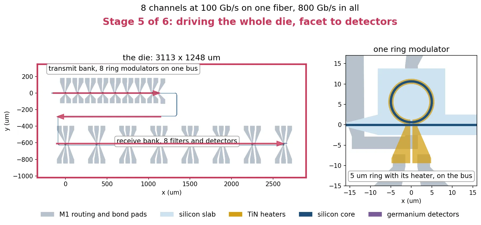
This notebook drives the eight-channel microring transceiver laid out in Chip Layout with real data and measures what comes out of it.

A comb of eight carriers enters the facet. Eight ring modulators, one per carrier, impress a 100 Gb/s pattern on each. The light crosses the die, eight coupled-ring drop filters separate the channels again, and eight photodiodes convert them back to voltage. The simulation is post layout: the component that is driven is the same chip object that produced the mask and passed the design rule check, with every route, taper, tap and bond-pad cell in place.

Three quantities have to be fixed before any of that can run.

The modulator bias detuning. A ring modulator transmits a minimum at resonance, and the slope of its transmission is zero there, so a ring driven exactly on resonance produces almost no modulation. The drive has to sit where the slope is steep, on the side of the resonance. How far to the side follows from the resonance shape, and the first cell below checks that the drive is small enough for that answer to hold.

The heater setting for all sixteen rings. The drawn ring sizes place each resonance near its channel but not on it, and the modulators additionally have to sit at the bias detuning above. Both corrections come from the heaters, whose efficiency was measured in Wavelength Plan and Thermal Budget.

The receiver bandwidth. The drop filters have to reject the neighbouring channel 200 GHz away and pass a 100 Gb/s signal at the same time. Component Library sizes them against both, and the last section here checks the finished chip against the same two numbers. That requirement came from this notebook: a filter chosen on crosstalk alone closed the eye, and only a link simulation showed it.

from runpy import run_path

# Optical_IO_Chip.qmd defines what this notebook builds on: everything measured so far.
# Its shared cells are generated into the module below; see
# docs/scripts/generate_notebook_modules.py.
globals().update(
    {k: v for k, v in run_path("misc/optical_io_chip.py").items() if not k.startswith("_")}
)

Operating point and simulation settings

The numbers below fall into three groups: the thermal calibration constants measured elsewhere, the optical and electrical operating point of the link, and the time step.

The thermal constants are read from misc/thermal_budget.npz, written by Wavelength Plan and Thermal Budget, so that this notebook does not repeat a HEAT solve. Two of them matter here: how many kelvin a milliwatt of heater power produces, and how many gigahertz a kelvin moves a resonance on each of the two waveguides.

The time step is set by the ring, not by the data. A time-domain circuit has to resolve the round trip inside the cavity, so the step is a fraction of that round trip, and the number of samples per bit follows from it rather than being chosen.

# Load the thermal results measured in Optical_IO_Thermal.ipynb
budget = np.load("misc/thermal_budget.npz")

# Take the heater efficiency, in kelvin of ring rise per milliwatt
k_per_mw = float(budget["k_per_mw"])

# Convert that to a resonance shift per milliwatt, for each waveguide type
ghz_per_mw_rib = k_per_mw * ghz_per_k_rib
ghz_per_mw_strip = k_per_mw * ghz_per_k_strip

t_ref = 293.0  # Temperature the component models were built at, K

# Calculate one round trip inside the modulator ring
tau_rt = 2 * np.pi * r_target * b["n_group"] / pf.C_0

# Set the time step to a quarter of a round trip, fine enough for the cavity
dt = tau_rt / 4

bit_rate = 100e9  # Line rate per channel
ui = int(round(1 / bit_rate / dt))  # Number of samples per bit
bit_rate = 1 / (ui * dt)  # Actual rate, after rounding to a whole sample count

z0 = 50.0  # Source impedance of the electrical ports
sq = np.sqrt(z0)  # Electrical wave amplitudes are volts over sqrt(z0)

v_drive = 3.0  # Modulator peak-to-peak drive voltage
p_line = 2e-3  # Input laser power per comb line: +3 dBm

# Work out how far the drive itself moves the resonance
drive_shift = (
    f0
    * abs(mod_kwargs["dn_dv"] * v_drive + mod_kwargs["dn_dv2"] * v_drive**2)
    / b["n_group"]
)

print(f"{'heater efficiency':24s} {k_per_mw:8.2f} K/mW")
print(f"{'modulator tuning':24s} {ghz_per_mw_rib:8.1f} GHz/mW")
print(f"{'filter tuning':24s} {ghz_per_mw_strip:8.1f} GHz/mW")
print(f"{'modulator linewidth':24s} {fwhm*1e-9:8.0f} GHz")
print(f"{'channel grid':24s} {channel_grid*1e-9:8.0f} GHz")
print(f"{'time step':24s} {dt*1e15:8.2f} fs")
print(f"{'samples per bit':24s} {ui:8d}")
print(f"{'line rate':24s} {bit_rate*1e-9:8.1f} Gb/s")
print(
    f"{'drive moves resonance':24s} {drive_shift*1e-9:8.0f} GHz "
    f"= {drive_shift/fwhm:.2f} linewidths"
)

heater efficiency            3.57 K/mW
modulator tuning             33.2 GHz/mW
filter tuning                30.8 GHz/mW
modulator linewidth           114 GHz
channel grid                  200 GHz
time step                  101.60 fs
samples per bit                98
line rate                   100.4 Gb/s
drive moves resonance          13 GHz = 0.11 linewidths

The drive moves the resonance by about a tenth of a linewidth, which is what the next section needs to know: the bias point below is derived for a drive small enough not to move the resonance at all.

Choosing the modulator bias detuning

For a drive that does not move the resonance, the optimum bias is where the transmission slope is steepest. For a Lorentzian dip that is its inflection point, at

$$\Delta f = \frac{\mathrm{FWHM}}{2\sqrt{3}} = 0.289\ \mathrm{linewidths}$$

which is the starting point used in the optical peaking example. The laser sits below the resonance, so each modulator is calibrated to hold its resonance that far above its own comb line.

A tenth of a linewidth of drive-induced shift is inside the range the formula is written for, so it is used as it stands. What says whether that was the right call is the eight eyes measured further down, and those are measured on the chip with all eight channels present. A sweep of one modulator on a bench cannot settle it: moving the bias further out improves a single ring, and at the same time raises the carrier of every neighbour, which is what the chip is actually limited by.

The two sides of the resonance are not equivalent either. A ring modulator chirps as it switches, because depleting the junction changes the loss as well as the index, and the sign of that interference depends on which side the laser sits. The laser is placed on the low-frequency side, which is the side the resonance itself moves toward as the junction depletes.

# Set the bias at the steepest slope, below the resonance
small_signal = fwhm / (2 * np.sqrt(3))
bias_detune = -small_signal

print(
    f"bias detuning {bias_detune*1e-9:.1f} GHz " f"= {bias_detune/fwhm:+.3f} linewidths"
)

bias detuning -33.0 GHz = -0.289 linewidths

The drive pattern and the eye metric

Every channel is driven with a maximal-length sequence of 31 bits, repeated three times, with the first period discarded so the cavities have filled before anything is measured. The pattern is short deliberately: run time scales with it, and the level transitions the eye is made of all appear within one period.

Two details of the eye metric matter. The two logic levels are separated using the bits that were sent, not by splitting the samples at their own average, which fails once the eye is nearly closed. And the sampling instant is searched rather than assumed, because the cavity and the 60 GHz detector together delay the waveform by a large part of a bit period, and the routing adds several whole bits on top. A real receiver recovers that instant from the data.

n_pattern = 31  # Bits in one period of the drive pattern
n_reps = 3  # Periods per run
n_bits = n_reps * n_pattern  # Bits per run
n_steps = n_bits * ui  # Total time steps per run
rise = max(1, int(round(0.3 * ui)))  # Rise and fall time, as a fraction of a bit

def prbs5(shift=0):
    """Generate the 31 bit maximal sequence of x^5 + x^3 + 1, rotated by shift."""
    reg, out = 0x1F, []
    for _ in range(n_pattern):
        bit = ((reg >> 4) ^ (reg >> 2)) & 1
        reg = ((reg << 1) | bit) & 0x1F
        out.append(bit)
    return np.roll(np.array(out), shift)

def nrz(bits):
    """Convert a bit sequence to a drive waveform with finite edges."""
    # Hold each bit for one symbol period
    level = np.repeat(np.tile(bits, n_reps), ui).astype(float)

    # Smooth the steps into ramps of the chosen rise time
    return np.convolve(level, np.ones(rise) / rise, mode="same") * v_drive

def eye_fold(v):
    """Fold a trace into overlapping two-bit segments for an eye diagram."""
    # Slide the window one bit at a time, so every transition lands mid trace
    n = len(v) // ui - 1
    return np.stack([v[k * ui : (k + 2) * ui] for k in range(n)])

def eye_q(v, bits, max_lag=24, instant=False):
    """Measure eye quality: level separation over level spread."""
    # Cut the trace into symbol periods
    keep = len(v) // ui
    blocks = v[: keep * ui].reshape(-1, ui)
    sent_all = np.tile(bits, n_reps)[-keep:]

    # Search over whole-bit lag as well, since the chip delays by several bits
    best, best_k = 0.0, 0
    for lag in range(max_lag):
        sent = np.roll(sent_all, lag)
        hi, lo = blocks[sent == 1], blocks[sent == 0]
        if len(hi) < 2 or len(lo) < 2:
            continue
        q = np.abs(hi.mean(axis=0) - lo.mean(axis=0)) / (
            hi.std(axis=0) + lo.std(axis=0) + 1e-18
        )
        k = int(np.argmax(q))
        if q[k] > best:
            best, best_k = float(q[k]), k

    # Return the sampling instant too, which is what an eye is centred on
    return (best, best_k) if instant else best

Setting the sixteen heaters

Each ring now has a target. A modulator has to sit at the measured bias detuning above its carrier. A filter has to sit centred on its carrier, where its drop port peaks.

Three facts make this a chip-level problem rather than sixteen independent ones.

The drawn sizes put each resonance near its channel but not on it, because the ring radii were snapped to the layout grid.

A heater can only heat, so it can only pull a resonance down in frequency. Every ring therefore has to start above where it must end up.

The comb is a rigid grid with one global position. A single laser offset has to give all sixteen rings room to be pulled down, and the ring furthest from its target sets that offset for everybody.

The heater setting itself enters the model as a temperature. The ring models carry a thermo-optic coefficient, so setting the ring temperature moves the resonance exactly as the heater would, and the same value feeds the frequency-domain model and the time stepper.

The calibration is measured rather than calculated. Each resonance is found on the cell that was actually built, the temperature is corrected, and it is measured again. This avoids two traps: a closed-form resonance formula holding the index fixed ignores dispersion, and a coupled pair has a flat passband whose peak is not a stable landmark, so filters are aligned by the centre of their passband instead.

One detail below is worth more than it looks. Every ring and every pass is measured on one shared frequency grid. PhotonForge solves a component’s port modes at each frequency it is asked for and caches the result on the frequency value, not on the component, so a grid centred on each channel in turn would pay a fresh mode solve per channel per pass. On this chip that one change is the difference between a section that takes minutes and one that takes an hour, and it changes no answer.

# Aim each modulator's resonance one bias detuning above its own comb line
bias_offset = -bias_detune

search = 400e9  # Half-width of the resonance search window, Hz
scan = np.arange(channel_freqs.min() - 600e9, channel_freqs.max() + 600e9, 5e9)
print(
    f"one scan of {len(scan)} frequencies, "
    f"{(scan[1]-scan[0])*1e-9:.0f} GHz apart, for all sixteen rings"
)

def dip_of(cell, key, guess, span=search):
    """Find the transmission minimum nearest a first estimate."""
    t = np.abs(cell.s_matrix(scan, show_progress=False)[key]) ** 2
    near = np.abs(scan - guess) < span
    return float(scan[np.flatnonzero(near)[np.argmin(t[near])]])

def band_centre_of(cell, key, guess, span=search):
    """Find the centre of a filter passband, as the midpoint of everything
    above half its peak."""
    t = np.abs(cell.s_matrix(scan, show_progress=False)[key]) ** 2
    near = np.abs(scan - guess) < span
    f, w = scan[near], t[near]
    inband = f[w >= 0.5 * w.max()]
    return float(0.5 * (inband.min() + inband.max()))

# Build one ring at a given temperature, for both device types
def warm_modulator(i, warm):
    """Modulator for channel i with its heater raising it warm kelvin."""
    return microring_modulator(
        **{**mod_kwargs, "ring_radius": mod_radius[i], "temperature": t_ref + warm}
    )

def warm_filter(i, warm):
    """Coupled-ring filter for channel i, likewise."""
    return two_ring_filter(
        **{
            **dict(second_order.parametric_kwargs),
            "coupling_length": drop_lc[i],
            "n_eff": n_eff_strip,
            "temperature": t_ref + warm,
        }
    )

# Measure where every cold resonance actually sits
mod_res = np.array(
    [
        dip_of(modulators[i], ("P0@0", "P1@0"), channel_freqs[i])
        for i in range(n_channels)
    ]
)
flt_res = np.array(
    [
        band_centre_of(filters[i], ("in@0", "drop@0"), channel_freqs[i])
        for i in range(n_channels)
    ]
)
print("cold resonances found")

# Offset the whole comb by what the most demanding ring needs
need = np.concatenate([channel_freqs - mod_res + bias_offset, channel_freqs - flt_res])
comb_offset = need.max() + 5e9  # 5 GHz of margin, so no heater sits at zero
laser_freqs = channel_freqs - comb_offset

# Estimate how far each heater has to pull its ring
mod_shift = mod_res - (laser_freqs + bias_offset)
flt_shift = flt_res - laser_freqs

# Convert that shift to the temperature which produces it
mod_warm = mod_shift * 1e-9 / ghz_per_k_rib
flt_warm = flt_shift * 1e-9 / ghz_per_k_strip

# Measure the warmed cell, correct the temperature, and measure again
for sweep in range(2):
    mod_err, flt_err = [], []
    for i in range(n_channels):
        want = laser_freqs[i] + bias_offset
        got = dip_of(warm_modulator(i, mod_warm[i]), ("P0@0", "P1@0"), want, span=150e9)
        mod_err.append(got - want)
        got = band_centre_of(
            warm_filter(i, flt_warm[i]), ("in@0", "drop@0"), laser_freqs[i], span=150e9
        )
        flt_err.append(got - laser_freqs[i])
        print(f"  pass {sweep}, channel {i} measured", flush=True)

    print(
        f"pass {sweep}: worst residual, modulator "
        f"{np.abs(mod_err).max()*1e-9:5.1f} GHz, filter "
        f"{np.abs(flt_err).max()*1e-9:5.1f} GHz"
    )

    # Fold the measured error back into the temperature
    mod_warm = mod_warm + np.array(mod_err) * 1e-9 / ghz_per_k_rib
    flt_warm = flt_warm + np.array(flt_err) * 1e-9 / ghz_per_k_strip

# Convert each temperature into the heater power it costs
mod_mw = mod_warm / k_per_mw
flt_mw = flt_warm / k_per_mw

print()
print(f"bias offset  {bias_offset*1e-9:.1f} GHz, resonance above the carrier")
print(f"comb offset  {comb_offset*1e-9:.1f} GHz, common to all eight lines")
print()
print(
    f"{'ch':>3s} {'laser THz':>10s} {'mod K':>7s} {'mod mW':>7s} "
    f"{'flt K':>7s} {'flt mW':>7s}"
)
for i in range(n_channels):
    print(
        f"{i:3d} {laser_freqs[i]*1e-12:10.4f} {mod_warm[i]:7.2f} "
        f"{mod_mw[i]:7.2f} {flt_warm[i]:7.2f} {flt_mw[i]:7.2f}"
    )
print()
print(
    f"tuning power {mod_mw.sum():.1f} mW transmit, {flt_mw.sum():.1f} mW "
    f"receive, {mod_mw.sum()+flt_mw.sum():.1f} mW total"
)
print(f"per ring     {np.concatenate([mod_mw, flt_mw]).mean():.2f} mW average")

one scan of 520 frequencies, 5 GHz apart, for all sixteen rings
cold resonances found
  pass 0, channel 0 measured
  pass 0, channel 1 measured
  pass 0, channel 2 measured
  pass 0, channel 3 measured
  pass 0, channel 4 measured
  pass 0, channel 5 measured
  pass 0, channel 6 measured
  pass 0, channel 7 measured
pass 0: worst residual, modulator   0.0 GHz, filter   2.0 GHz
  pass 1, channel 0 measured
  pass 1, channel 1 measured
  pass 1, channel 2 measured
  pass 1, channel 3 measured
  pass 1, channel 4 measured
  pass 1, channel 5 measured
  pass 1, channel 6 measured
  pass 1, channel 7 measured
pass 1: worst residual, modulator   0.0 GHz, filter   3.0 GHz

bias offset  33.0 GHz, resonance above the carrier
comb offset  48.0 GHz, common to all eight lines

 ch  laser THz   mod K  mod mW   flt K  flt mW
  0   192.6665    0.54    0.15    5.09    1.43
  1   192.8665    1.07    0.30    5.96    1.67
  2   193.0665    1.61    0.45    5.67    1.59
  3   193.2665    2.15    0.60    5.67    1.59
  4   193.4665    0.54    0.15    5.38    1.51
  5   193.6665    1.07    0.30    5.38    1.51
  6   193.8665    2.15    0.60    5.67    1.59
  7   194.0665    2.68    0.75    5.67    1.59

tuning power 3.3 mW transmit, 12.5 mW receive, 15.8 mW total
per ring     0.99 mW average

The first pass already lands every ring within the scan step, and the second returns the same numbers. That is not luck: the cold resonance is measured rather than predicted, and a ring model’s resonance moves exactly linearly with its temperature, so one measurement and one division is the whole correction. The second pass is the check that says so, and it costs nothing now that the grid is shared. Either way the residual is far inside both the modulator linewidth and the filter passband, so every ring is on its channel.

The filters cost more power than the modulators, for two reasons. Their straight sections were snapped to a coarser grid, so they start further from their targets, and they carry the full comb offset while the modulators get part of it back as their bias detuning.

The milliwatt figures use the kelvin per milliwatt measured on the modulator’s heater, which is the only one Wavelength Plan and Thermal Budget solved. A filter heater is narrower, and a narrower heater puts the same power into a smaller volume directly over the mode, so its real efficiency is a little better and these numbers are an upper bound. The calibration itself is unaffected, because it works in temperature.

The plots below show the result directly: eight modulator resonances, each sitting the bias detuning above its carrier, and eight filter passbands, each centred on one.

# Build the calibrated cells once, for the plots and the chip alike
mods_cal = [warm_modulator(i, mod_warm[i]) for i in range(n_channels)]
flts_cal = [warm_filter(i, flt_warm[i]) for i in range(n_channels)]

# Scan a window spanning all eight channels, with room either side
span = np.linspace(laser_freqs.min() - 300e9, laser_freqs.max() + 300e9, 401)

fig, ax = plt.subplots(2, 1, figsize=(10, 5.5), sharex=True, tight_layout=True)

# Plot each modulator's through-port transmission
for i in range(n_channels):
    t = np.abs(mods_cal[i].s_matrix(span, show_progress=False)[("P0@0", "P1@0")]) ** 2
    ax[0].plot((span - f0) * 1e-12, 10 * np.log10(t), lw=1)

# Plot each filter's drop-port transmission
for i in range(n_channels):
    d = np.abs(flts_cal[i].s_matrix(span, show_progress=False)[("in@0", "drop@0")]) ** 2
    ax[1].plot((span - f0) * 1e-12, 10 * np.log10(d), lw=1)

# Mark the comb lines, which is what both rows are aligned to
for a in ax:
    for fl in laser_freqs:
        a.axvline((fl - f0) * 1e-12, color="gray", ls=":", lw=0.8)
    a.grid(True, alpha=0.3)
ax[0].set(
    ylabel="through (dB)",
    ylim=(-25, 2),
    title="calibrated modulators, biased off their carriers",
)
ax[1].set(
    xlabel="frequency offset from the design carrier (THz)",
    ylabel="drop (dB)",
    ylim=(-40, 2),
    title="calibrated demultiplexer, centred on the carriers",
)
plt.show()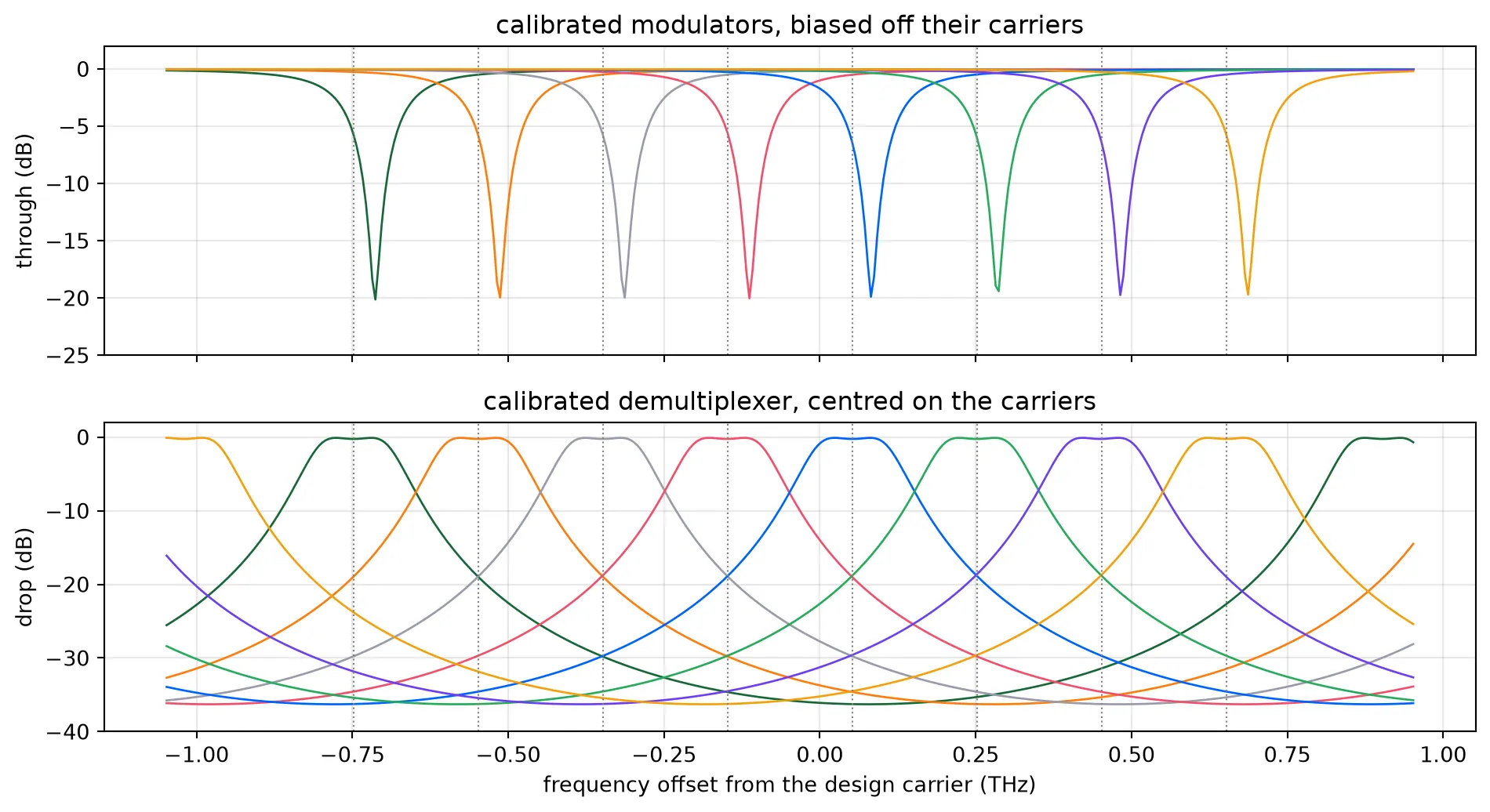

Simulating the full chip

The calibration is applied by rebuilding the chip with the warmed rings. The bank and die assembly from Chip Layout is reused directly, so what is simulated has the same routes, tapers, monitor tap, bond pads and hierarchy as the mask, with only the ring temperatures changed.

All eight channels are modulated at once, in a single run. The stimulus is a comb of eight tones on the fibre port and eight independent drive patterns, one per modulator, stepped together through one ts.step call. Each channel carries a different rotation of the sequence, so neighbours are never sending the same bits at the same time, and the eight detectors are read together. The eye diagrams below therefore already contain whatever the other seven channels do to each one: carrier crosstalk through the filters, and any interaction between modulators sharing the bus.

# Rebuild both banks with the calibrated rings and assemble the die
tx_cal, _, _ = build_tx_bank([mrm_with_bond_pads(modulator=m) for m in mods_cal])
rx_cal, _, _ = build_rx_bank([filter_with_bond_pads(filter_cell=f) for f in flts_cal])
chip_cal = assemble_chip(tx_cal, rx_cal)

print(
    f"simulating {chip_cal.name}, footprint "
    f"{chip_cal.size()[0]:.0f} x {chip_cal.size()[1]:.0f} um"
)

# One rotation of the pattern per channel, so the lanes are decorrelated
lane_bits = {i: prbs5(shift=7 * i) for i in range(n_channels)}

# Put the carrier in the middle of the comb so the baseband spans it evenly
f_carrier = laser_freqs[n_channels // 2]

# Build the input comb as a sum of tones about the carrier
t = np.arange(n_steps) * dt
comb = sum(
    np.sqrt(p_line) * np.exp(-2j * np.pi * (fl - f_carrier) * t) for fl in laser_freqs
)

# Feed the comb to the fibre port and its own pattern to each drive port
inputs = {"FIBER@0": np.asarray(comb, dtype=complex)}
for i in range(n_channels):
    inputs[f"DRIVE{i}@0"] = nrz(lane_bits[i]) / sq

# Step the whole chip
ts = chip_cal.setup_time_stepper(
    time_step=dt, carrier_frequency=f_carrier, show_progress=True
)
out = ts.step(inputs=pf.TimeSeries(inputs, dt), show_progress=True)

# Discard the first pattern period, during which the cavities fill
rx = {i: (np.real(out[f"RX{i}@0"]) * sq)[n_pattern * ui :] for i in range(n_channels)}

print()
print(f"{'ch':>3s} {'mean mV':>9s} {'eye Q':>7s}")
for i in range(n_channels):
    print(f"{i:3d} {rx[i].mean()*1e3:9.3f} {eye_q(rx[i], lane_bits[i]):7.2f}")

simulating optical_io_chip, footprint 3113 x 1248 um
Uploading task 'Mode-Ribwaveguideon90nmslabTE500nm…'
Uploading task 'Mode-Ribwaveguideon90nmslabTE500nm…'
Uploading task 'Mode-StripwaveguideTE500nm…'
Uploading task 'Mode-StripwaveguideTE500nm…'
Starting task 'Mode-Ribwaveguideon90nmslabTE500nm': https://tidy3d.simulation.cloud/workbench?taskId=mo-5b403463-34dd-42ad-9173-dd80d904ec12
Starting task 'Mode-Ribwaveguideon90nmslabTE500nm': https://tidy3d.simulation.cloud/workbench?taskId=mo-91e192e3-b5ee-4b59-8ce8-c9a5cd996c69
Downloading data from 'Mode-Ribwaveguideon90nmslabTE500nm'…
Downloading data from 'Mode-Ribwaveguideon90nmslabTE500nm'…
Starting task 'Mode-StripwaveguideTE500nm': https://tidy3d.simulation.cloud/workbench?taskId=mo-82c8e5bd-d8b2-4139-9027-169e15e7c5d7
Starting task 'Mode-StripwaveguideTE500nm': https://tidy3d.simulation.cloud/workbench?taskId=mo-dc7774cd-0598-4bcd-a203-2a56cefad1aa
Uploading task 'Mode-StripwaveguideTE500nm…'
Uploading task 'Mode-StripwaveguideTE500nm…'
Downloading data from 'Mode-StripwaveguideTE500nm'…
Downloading data from 'Mode-StripwaveguideTE500nm'…
Starting task 'Mode-StripwaveguideTE500nm': https://tidy3d.simulation.cloud/workbench?taskId=mo-8d8e2eb8-e80b-4ef5-b0cb-859a681e1ff1
Starting task 'Mode-StripwaveguideTE500nm': https://tidy3d.simulation.cloud/workbench?taskId=mo-9fa7b336-21bc-45a7-a2f8-f3a34977e2e0
Downloading data from 'Mode-StripwaveguideTE500nm'…
Downloading data from 'Mode-StripwaveguideTE500nm'…

 ch   mean mV   eye Q
  0   168.008    7.51
  1   155.512    4.89
  2   158.163    5.63
  3   162.952    5.34
  4   121.218    5.27
  5   124.855    6.39
  6    93.403    4.72
  7    98.909    6.70

Every channel receives power and every channel carries its own data, so the wavelength plan, the calibration and the routing are all consistent.

What sets the eye quality here is no longer the receive filter, which passes the signal with room to spare. It is the other seven channels. Each one is rejected by the figure measured at the end of this notebook, not removed, and seven of them arrive together, so the crosstalk that reaches a detector sits only about ten decibels below the channel it is trying to read. Neither a filter response on its own nor a single modulator driven into a bare photodiode shows that.

probe_ch = n_channels // 2  # Channel used for the single-lane comparison

# Build a time axis two bit periods wide, centred on a transition
t_eye = (np.arange(2 * ui) - ui) * dt * 1e12

# One eye per channel, in two rows of four
fig, ax = plt.subplots(2, 4, figsize=(13, 6), tight_layout=True)
for i, a in enumerate(ax.ravel()):

    # Roll each trace so the sampling instant lands in the middle
    q, k = eye_q(rx[i], lane_bits[i], instant=True)

    # Overlay every two-bit segment of the detected trace
    a.plot(
        t_eye, eye_fold(np.roll(rx[i], -k)).T * 1e3, color="#1f4e79", lw=0.8, alpha=0.45
    )
    a.grid(True, alpha=0.2)
    a.set(title=f"channel {i} (Q = {q:.2f})")
for a in ax[1]:
    a.set_xlabel("time (ps)")
for a in ax[:, 0]:
    a.set_ylabel("detected voltage (mV)")
plt.show()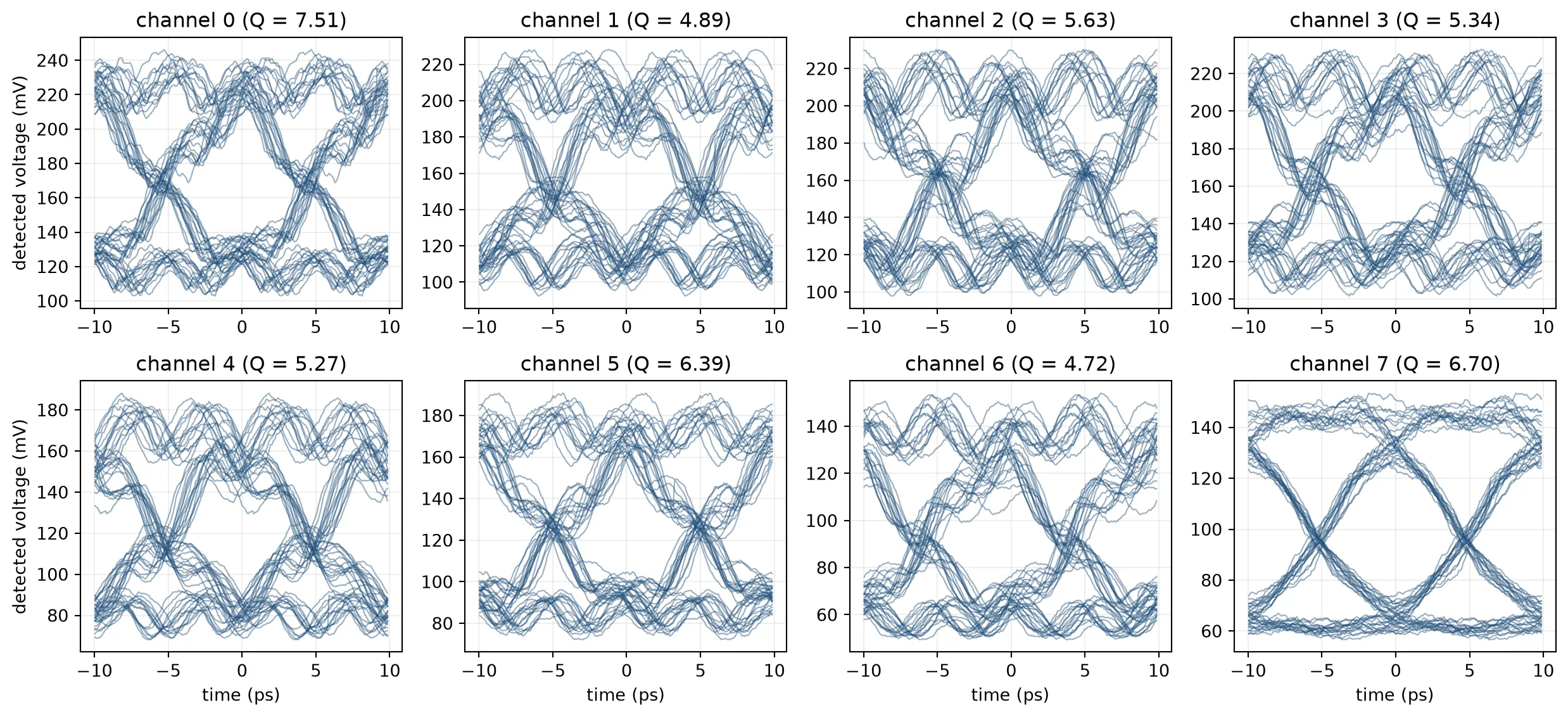

What the other seven channels cost

The eyes above are measured with every channel modulating. Two more runs separate what the neighbours cost by modulating from what they cost by being there at all. The first keeps the full comb and drives one lane, holding the other seven at zero. The second also removes the other seven carriers, leaving one tone and one modulated channel.

def drive_chip(carriers, lanes):
    """Drive the calibrated chip and return one channel's detected trace.

    'carriers' is the optical input, 'lanes' the channels that modulate.
    """
    inputs = {"FIBER@0": np.asarray(carriers, dtype=complex)}
    for i in range(n_channels):
        pattern = nrz(lane_bits[i]) if i in lanes else np.zeros(n_steps)
        inputs[f"DRIVE{i}@0"] = pattern / sq

    # A fresh stepper each time, so no state carries over between runs
    stepper = chip_cal.setup_time_stepper(
        time_step=dt, carrier_frequency=f_carrier, show_progress=True
    )
    detected = stepper.step(inputs=pf.TimeSeries(inputs, dt), show_progress=True)
    return (np.real(detected[f"RX{probe_ch}@0"]) * sq)[n_pattern * ui :]

# One tone on the probe channel, instead of the eight-line comb
one_tone = np.sqrt(p_line) * np.exp(
    -2j * np.pi * (laser_freqs[probe_ch] - f_carrier) * t
)

traces = {
    "eight carriers, eight modulating": rx[probe_ch],
    "eight carriers, one modulating": drive_chip(comb, {probe_ch}),
    "one carrier, one modulating": drive_chip(one_tone, {probe_ch}),
}

print(f"channel {probe_ch}")
print(f"{'':36s} {'eye Q':>7s} {'mean mV':>9s}")
for label, trace in traces.items():
    print(
        f"{label:36s} {eye_q(trace, lane_bits[probe_ch]):7.2f} "
        f"{trace.mean()*1e3:9.1f}"
    )

channel 4
                                       eye Q   mean mV
eight carriers, eight modulating        5.27     121.2
eight carriers, one modulating          5.19     121.0
one carrier, one modulating             7.68     118.2

# The three eyes side by side, on shared axes
fig, ax = plt.subplots(1, 3, figsize=(13, 3.6), tight_layout=True, sharey=True)
for a, (label, trace) in zip(ax, traces.items()):
    q, k = eye_q(trace, lane_bits[probe_ch], instant=True)
    a.plot(
        t_eye, eye_fold(np.roll(trace, -k)).T * 1e3, color="#1f4e79", alpha=0.25, lw=0.7
    )
    a.set_title(f"{label}\nQ = {q:.2f}", fontsize=9)
    a.set_xlabel("time (ps)")
    a.grid(alpha=0.3)
ax[0].set_ylabel("detected (mV)")
plt.show()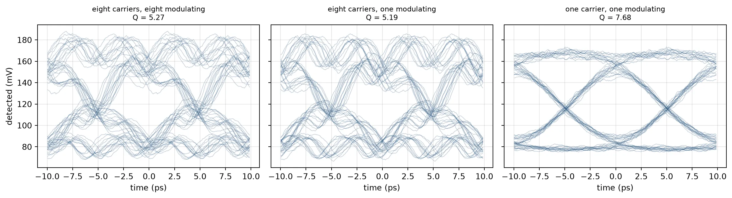

Modulating the neighbours does not measurably change the eye. What costs is their presence: removing the other seven carriers takes this channel from Q 5.1 to Q 7.7.

The reason is that a photodiode adds fields, not powers. The leaked carriers raise the mean by about 3 mV, which is their power at the 18.6 dB of rejection measured below. They also beat against the wanted signal, and that term goes as the square root of the two powers, so an 18.6 dB power leak is a 9.3 dB beat. It lands at the 200 GHz channel spacing, where the first-order 60 GHz detector still passes about a quarter of it.

The beat is visible in the first two eyes: the traces carry an oscillation about 5 ps long, which is one period at the channel spacing, so the rails are rippled rather than blurred. The third eye has nothing left to beat against, and its rails are flat.

That also explains why modulation makes no difference. The beat follows the leaked carrier amplitude, which is there whether or not the neighbour carries data.

The chip’s own spectrum

Everything above was measured on a waveform. The same calibrated chip can also be swept, which puts every resonance and every laser line on one axis and shows where the light actually goes.

The figure has three rows.

The receive bus, from the fibre to the far end. Each channel puts two notches on it rather than one, which is not obvious and is worth an explanation. The third row gives it.

Every channel output, all eight on one axis. The photodiodes take the drop ports, so those are not available as optical outputs on the chip that was driven. The same chip is therefore assembled once more with the detectors left off, which exposes each channel’s drop directly. Nothing else about it changes, so this is the same eight paths the waveform took.

One channel, magnified, with the bus trace laid over the two rings’ own through responses. This is the row that says which notch is which.

# Sweep the same assembled chip from the fibre port, on the calibration's grid
probe = scan[np.abs(scan - laser_freqs.mean()) < 0.5 * channel_span + 400e9]
s_chip = chip_cal.s_matrix(
    probe, model_kwargs={"inputs": ["FIBER"]}, show_progress=True
)

# Rebuild the chip without detectors, so each drop becomes an optical port
rx_probe, _, _ = build_rx_bank(
    [filter_with_bond_pads(filter_cell=f, detector=False) for f in flts_cal],
    name="rx_bank_probe",
)
s_probe = assemble_chip(tx_cal, rx_probe, name="optical_io_chip_probe").s_matrix(
    probe, model_kwargs={"inputs": ["FIBER"]}, show_progress=True
)

# Take the light left on the receive bus once all eight have been dropped
thru = np.abs(s_chip[("FIBER@0", "RX_THRU@0")]) ** 2

# Cut one channel's worth of frequency out, for the magnified row
mid = n_channels // 2
near = np.abs(probe - laser_freqs[mid]) < 0.7 * channel_grid
off = (probe[near] - laser_freqs[mid]) * 1e-9

fig, ax = plt.subplots(3, 1, figsize=(11, 9.5), tight_layout=True)

# Plot the receive bus end to end
ax[0].plot((probe - f0) * 1e-12, 10 * np.log10(thru), lw=1.8, color="#1f4e79")

# Plot fibre to each channel's own output, all eight together
for i in range(n_channels):
    out = np.abs(s_probe[("FIBER@0", f"RX{i}@0")]) ** 2
    ax[1].plot((probe - f0) * 1e-12, 10 * np.log10(out), lw=1.6, label=f"ch {i}")
ax[1].legend(fontsize=8, ncol=8, loc="lower center")

# Mark the comb on both wide rows
for a in ax[:2]:
    for fl in laser_freqs:
        a.axvline((fl - f0) * 1e-12, color="crimson", lw=0.7, alpha=0.7)

    # Hold the view to the comb, clear of the free spectral range repeats
    a.set_xlim(
        (laser_freqs.min() - f0 - 250e9) * 1e-12,
        (laser_freqs.max() - f0 + 250e9) * 1e-12,
    )

# Plot the same bus trace over one channel, against what each ring does alone
ax[2].plot(
    off,
    10 * np.log10(thru[near] / thru.max()),
    lw=2.4,
    color="#1f4e79",
    label="the receive bus",
)
mod_t = (
    np.abs(mods_cal[mid].s_matrix(probe[near], show_progress=False)[("P0@0", "P1@0")])
    ** 2
)
flt_t = (
    np.abs(flts_cal[mid].s_matrix(probe[near], show_progress=False)[("in@0", "thru@0")])
    ** 2
)
ax[2].plot(
    off,
    10 * np.log10(mod_t),
    lw=1.6,
    ls="--",
    color="#c8385a",
    label="its modulator alone",
)
ax[2].plot(
    off, 10 * np.log10(flt_t), lw=1.6, ls=":", color="#3aa596", label="its filter alone"
)
ax[2].axvline(0, color="crimson", lw=0.9, label="the laser line")
ax[2].legend(fontsize=9, loc="lower right")

# Print where each ring actually puts its notch
print(
    f"filter notches at {off[off < 0][np.argmin(flt_t[off < 0])]:+.0f} and "
    f"{off[off > 0][np.argmin(flt_t[off > 0])]:+.0f} GHz from the line"
)
print(
    f"modulator dip at {off[np.argmin(mod_t)]:+.0f} GHz, "
    f"{10*np.log10(mod_t.min()):.1f} dB deep"
)

for a in ax:
    a.grid(True, alpha=0.25)
ax[0].set(
    ylabel="bus transmission (dB)",
    ylim=(-45, 2),
    title="fibre to the far end of the receive bus",
)
ax[1].set(
    ylabel="channel output (dB)",
    ylim=(-45, 2),
    title="fibre to each of the eight channel outputs",
)
ax[2].set(
    xlabel=f"offset from channel {mid}'s laser line (GHz)",
    ylabel="normalised (dB)",
    ylim=(-40, 2),
    title="one channel, magnified: which notch belongs to which ring",
)
plt.show()

# Print what is left of each comb line, and what reaches its own detector
print(f"{'ch':>3s} {'left on the bus':>16s} {'at its output':>14s}")
for i in range(n_channels):
    out = np.abs(s_probe[("FIBER@0", f"RX{i}@0")]) ** 2
    print(
        f"{i:3d} {10*np.log10(np.interp(laser_freqs[i], probe, thru)/thru.max()):13.1f} dB"
        f" {10*np.log10(np.interp(laser_freqs[i], probe, out)):11.1f} dB"
    )

Uploading task 'Mode-Ribwaveguideon90nmslabTE500nm…'
Uploading task 'Mode-Ribwaveguideon90nmslabTE500nm…'
Uploading task 'Mode-StripwaveguideTE500nm…'
Uploading task 'Mode-StripwaveguideTE500nm…'
Uploading task 'Mode-StripwaveguideTE500nm…'
Uploading task 'Mode-StripwaveguideTE500nm…'
Starting task 'Mode-Ribwaveguideon90nmslabTE500nm': https://tidy3d.simulation.cloud/workbench?taskId=mo-e7061a66-3744-4ac7-b7ae-9a64c4ecc452
Starting task 'Mode-StripwaveguideTE500nm': https://tidy3d.simulation.cloud/workbench?taskId=mo-934a1d0d-b533-496b-b0a0-62e55792bbc1
Starting task 'Mode-Ribwaveguideon90nmslabTE500nm': https://tidy3d.simulation.cloud/workbench?taskId=mo-c196f68d-5651-4455-9d32-4b7f9776cf0e
Starting task 'Mode-StripwaveguideTE500nm': https://tidy3d.simulation.cloud/workbench?taskId=mo-2f831df2-7a37-4eb9-9b82-9ad2f3cd26fe
Starting task 'Mode-StripwaveguideTE500nm': https://tidy3d.simulation.cloud/workbench?taskId=mo-f7a23b6a-0ccd-4805-869d-71d835b57565
Starting task 'Mode-StripwaveguideTE500nm': https://tidy3d.simulation.cloud/workbench?taskId=mo-927aa946-5522-4f06-a9bb-ca690fc3d92c
Downloading data from 'Mode-Ribwaveguideon90nmslabTE500nm'…
Downloading data from 'Mode-StripwaveguideTE500nm'…
Downloading data from 'Mode-Ribwaveguideon90nmslabTE500nm'…
Downloading data from 'Mode-StripwaveguideTE500nm'…
Downloading data from 'Mode-StripwaveguideTE500nm'…
Downloading data from 'Mode-StripwaveguideTE500nm'…
filter notches at -27 and +28 GHz from the line
modulator dip at +33 GHz, -19.4 dB deep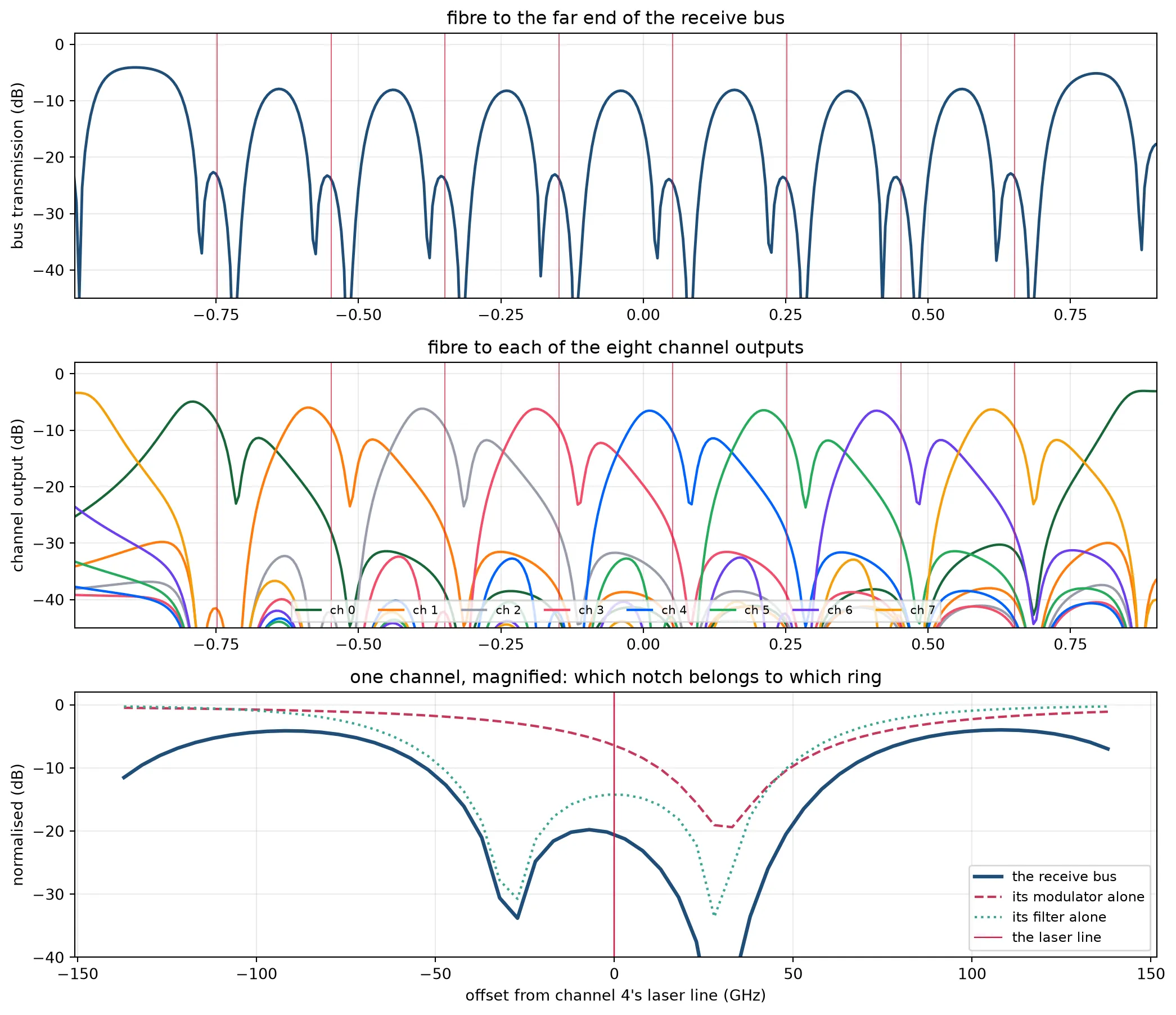

 ch  left on the bus  at its output
  0         -19.2 dB        -8.7 dB
  1         -19.8 dB        -9.4 dB
  2         -19.9 dB        -9.5 dB
  3         -19.8 dB        -9.5 dB
  4         -20.6 dB       -10.4 dB
  5         -20.1 dB       -10.0 dB
  6         -20.5 dB       -10.4 dB
  7         -19.5 dB        -9.6 dB

The magnified row answers the question the wide one raises, and the answer is not the obvious one. Both notches belong to the filter.

A series-coupled pair has two supermodes, so it drops over a band rather than at a line, and its through port has two minima, one at each edge of that band. They are what the wide row shows, and they are deep because at those two frequencies the filter has taken almost everything off the bus. The modulator is the shallow feature between them, about 20 dB deep and parked the bias detuning above the line so that its flank rather than its floor does the modulating. On the bus it is swallowed by the filter’s own notch.

This is worth knowing before a measurement rather than after one. A probe station sweeping the through port of one of these channels sees a pair of notches per channel, and reading either of them as a resonance to be centred on the laser would put the filter in the wrong place.

The middle row is the demultiplexer doing its job seen end to end: eight passbands, each on its own line, each carrying the loss of the facet, the modulators it passed, the monitor tap and the millimetres of routing between the banks.

Demultiplexer bandwidth against the data rate

The receive filter has to satisfy two requirements that act on the same quantity. It must be narrow enough that the neighbouring channel, 200 GHz away, is rejected, and wide enough that a 100 Gb/s signal passes without distortion. The measurement below puts both on one axis: the drop response of the calibrated filter, with the signal bandwidth shaded and the neighbouring channel positions marked.

# Sweep one calibrated filter's drop, out past the neighbouring channels
probe = laser_freqs[n_channels // 2] + np.linspace(-1.5, 1.5, 121) * channel_grid
drop = (
    np.abs(
        flts_cal[n_channels // 2].s_matrix(probe, show_progress=False)[
            ("in@0", "drop@0")
        ]
    )
    ** 2
)

# Take everything within 3 dB of the peak, whose span is the passband
inband = probe[drop >= 0.5 * drop.max()]
width = inband.max() - inband.min()

# Sample at the channel itself and at its neighbour
centre = int(np.argmin(np.abs(probe - laser_freqs[n_channels // 2])))
adjacent = int(np.argmin(np.abs(probe - laser_freqs[n_channels // 2] - channel_grid)))

fig, ax = plt.subplots(figsize=(7.5, 3.4), tight_layout=True)

# Plot the drop response against offset from the channel
ax.plot((probe - laser_freqs[n_channels // 2]) * 1e-9, 10 * np.log10(drop), lw=1.3)

# Shade the bandwidth a 100 Gb/s NRZ signal occupies
ax.axvspan(
    -bit_rate * 1e-9 / 2,
    bit_rate * 1e-9 / 2,
    color="tab:orange",
    alpha=0.18,
    label=f"{bit_rate*1e-9:.0f} Gb/s signal",
)
for sign in (-1, 1):
    ax.axvline(
        sign * channel_grid * 1e-9,
        color="crimson",
        ls="--",
        lw=1,
        label="neighbouring channel" if sign > 0 else None,
    )
ax.set(
    xlabel="offset from the channel (GHz)",
    ylabel="drop transmission (dB)",
    ylim=(-45, 2),
    title="demultiplexer passband and the signal it carries",
)
ax.legend(fontsize=8)
ax.grid(True, alpha=0.3)
plt.show()

print(f"passband, 3 dB width    {width*1e-9:6.0f} GHz")
print(f"signal bandwidth        {bit_rate*1e-9:6.0f} GHz")
print(f"rejection one channel away {10*np.log10(drop[centre]/drop[adjacent]):5.1f} dB")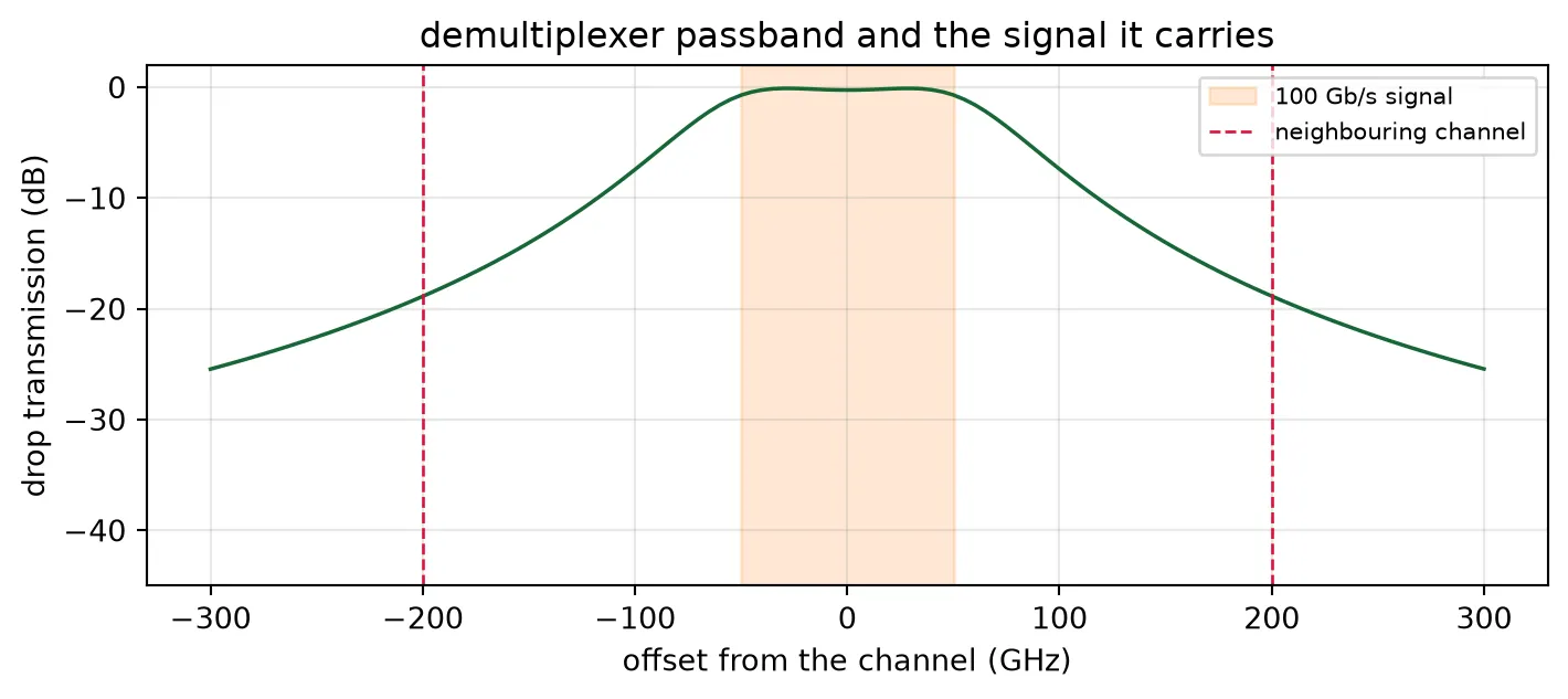

passband, 3 dB width       140 GHz
signal bandwidth           100 GHz
rejection one channel away  18.6 dB

Both requirements are satisfied, with little to spare. The passband is wider than the signal, so the signal passes, and the neighbouring channel is close to 20 dB down.

This is the requirement that a link simulation creates. An earlier version of this filter was a cascade of two independent add-drop rings, and it was chosen on its crosstalk figure alone: 74 GHz of passband with 21.7 dB of rejection. On paper that is the better filter. Driven with data it closed the eye on every channel, because a 74 GHz passband removes most of the spectrum of a 100 Gb/s signal, and no frequency-domain check of the filter, the modulator or the layout showed it.

The reason a cascade cannot do better is its shape. Two add-drop rings in series multiply two Lorentzians, so the skirts still fall at one ring’s rate: every gigahertz of passband bought back costs the rejection it bought. Coupling the two rings to each other makes the filter second order instead. Its skirts fall twice as fast, so the same rejection arrives at nearly twice the width, which is what the eyes above are worth.

What limits the link now is the rejection rather than the passband. Seven neighbours arrive at the figure printed above, and that, not the modulator and not the routing, is what sets the eye quality the chip reaches. A third ring, or a wider channel grid, is where the next improvement comes from.

Link budget

Each term below was measured somewhere in the series. The optical budget is a product of scalars, so the power it predicts at the detector can be compared with the power the time-domain run delivered.

# Measure one biased modulator's loss at its own carrier, undriven
f_ch = [laser_freqs[n_channels // 2]]
tx_il = -10 * np.log10(
    np.abs(
        mods_cal[n_channels // 2].s_matrix(f_ch, show_progress=False)[("P0@0", "P1@0")]
    )[0]
    ** 2
)

# Measure what the same carrier loses passing the other seven
idle_il = sum(
    -10
    * np.log10(
        np.abs(mods_cal[i].s_matrix(f_ch, show_progress=False)[("P0@0", "P1@0")])[0]
        ** 2
    )
    for i in range(n_channels)
    if i != n_channels // 2
)

# Measure the loss at the centre of the filter that drops this channel
rx_il = -10 * np.log10(drop[centre])

# Measure the waveguide length between the banks, which carries the routing loss
link_um = sum(
    pf.route_length(r.component)
    for r in chip_cal.references
    if "route" in str(r.component.parametric_function or "")
)

terms = [
    ("comb line at the facet", 10 * np.log10(p_line * 1e3), "dBm"),
    ("facet coupling", -1.5, "dB"),
    ("its own modulator", -tx_il, "dB"),
    ("seven idle modulators", -idle_il, "dB"),
    ("monitor tap", -0.05, "dB"),
    (f"on-chip link, {link_um:.0f} um", -scattering_db_cm * 1e-4 * link_um, "dB"),
    ("demultiplexer drop", -rx_il, "dB"),
]
total = sum(v for _, v, _ in terms)

print(f"{'term':28s} {'value':>9s}")
for name, v, unit in terms:
    print(f"{name:28s} {v:9.2f} {unit}")
print("-" * 40)
print(f"{'received power':28s} {total:9.2f} dBm")

# Compare the budget with the run, through the detector responsivity and gain
p_rx = 10 ** (total / 10) * 1e-3
print()
print(f"budget predicts   {p_rx*0.9*1e6:8.2f} uA")
print(f"simulation gives  {rx[n_channels//2].mean()/1e3*1e6:8.2f} uA")

term                             value
comb line at the facet            3.01 dBm
facet coupling                   -1.50 dB
its own modulator                -6.42 dB
seven idle modulators            -1.10 dB
monitor tap                      -0.05 dB
on-chip link, 2352 um            -0.47 dB
demultiplexer drop               -0.26 dB
----------------------------------------
received power                   -6.79 dBm

budget predicts     188.48 uA
simulation gives    121.22 uA

The two disagree, and the direction is informative. The budget is a single-frequency calculation on an undriven chip: it takes each modulator’s transmission at its bias point and multiplies. In the run every modulator is swinging, this channel’s and the seven it passes on the way out, and the mean transmission of a ring sweeping across its own flank is not the transmission at the bias point. A budget made of scalars has nowhere to put that.

Power and energy per bit

The optical power is set by the comb, the electrical power by the drivers and the heaters.

# Add up the aggregate rate across all channels
line_rate = n_channels * bit_rate

# Work out the driver power, a CV^2/4 cost per channel on a random pattern
p_driver = 0.25 * c_junction * 1e-15 * v_drive**2 * bit_rate * n_channels

# Take the heater power from the calibration above
p_tuning = (mod_mw.sum() + flt_mw.sum()) * 1e-3

# Add up the optical power launched into the chip
p_optical = n_channels * p_line

print(f"{'':22s} {'mW':>9s} {'fJ/bit':>9s}")
for name, p in (
    ("comb, on chip", p_optical),
    ("drivers", p_driver),
    ("heaters", p_tuning),
):
    print(f"{name:22s} {p*1e3:9.2f} {p/line_rate*1e15:9.1f}")
print("-" * 42)
total_p = p_optical + p_driver + p_tuning
print(f"{'total':22s} {total_p*1e3:9.2f} {total_p/line_rate*1e15:9.1f}")
print()
print(f"per channel {bit_rate*1e-9:.1f} Gb/s, {line_rate*1e-12:.3f} Tb/s per fibre")

                              mW    fJ/bit
comb, on chip              16.00      19.9
drivers                    32.97      41.0
heaters                    15.78      19.6
------------------------------------------
total                      64.75      80.6

per channel 100.4 Gb/s, 0.803 Tb/s per fibre

Summary

An eight-channel microring transceiver on 220 nm silicon, simulated post layout from the same component that produced the mask.

Line rate	8 channels at 100 Gb/s on a 200 GHz grid
Die	3113 x 1248 um, 3.88 mm2, design rule clean
Modulator	5 um ring, 113 GHz linewidth, biased 0.289 linewidths off resonance
Demultiplexer	two series-coupled racetracks per channel, flat top
Tuning	measured heater efficiency, sixteen rings calibrated by temperature
Monitor	one 1 percent tap and photodiode at the transmit output

Four solvers fed one circuit. FDTD set the coupling gaps and the waveguide transitions, mode solving gave every index and the thermo-optic shift, CHARGE gave the junction its efficiency and its loss, HEAT gave the kelvin per milliwatt the tuning budget rests on, and the circuit simulator turned all of it into a waveform.

Two results could only come from the link, and neither is visible in a layout or in a frequency-domain check of any single component.

The wavelength plan had been drawn with a fixed index where the group index was needed, which placed the eight resonances on the wrong comb spacing.

The demultiplexer had to be redesigned. Selected on its crosstalk figure alone, it was a cascade of two independent rings whose passband was narrower than the data rate it carried, and it closed the eye on every channel. A crosstalk figure carries no information about data rate. Coupling the two rings to each other makes the filter second order, which allows one passband to be wide enough for the signal and steep enough for the neighbour.