Volume Mesher#
The Volume Mesher generates a volume mesh from a surface mesh. It grows prism layers from the surface and fills the farfield with an octree-based mesh, connected by a layer of tetrahedra. It is currently opt-in: enable it via the beta mesher toggle in both the WebUI and the Python API (see Meshing for how the beta mesher and GAI toggles select each meshing workflow).
Available features:
Boundary layers:
per-face first-layer thickness and growth rate
automatic boundary-layer count from a target wall spacing
boundary-layer projection onto planar and axisymmetric surfaces
selective disabling of boundary-layer growth per face
Refinements:
uniform volumetric refinements using cylinders or boxes
axisymmetric volumetric refinements using cylinders
Zones:
axisymmetric zones with interfaces
custom volumetric zones defined by their enclosing surfaces
automatic farfield zone generation (sphere or semi-sphere, sized from the geometry bounding box)
structured mesh regions for porous media.
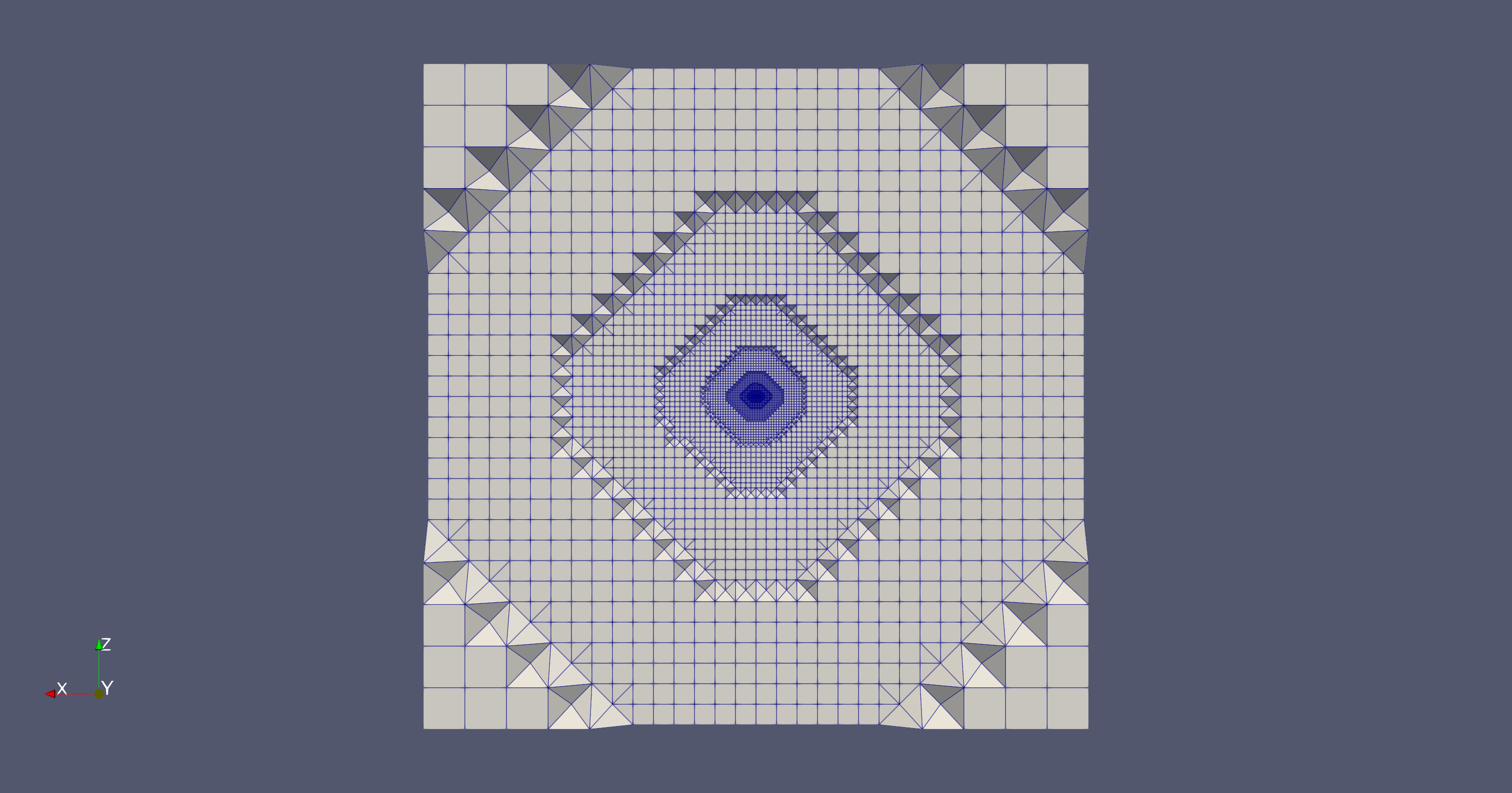
Clip of an example mesh generated using the Volume Mesher.#
Boundary layer behaviour#
By default, the Volume Mesher grows the prism stack from each wall until the top cells reach near-isotropy (aspect ratio ~1). The layer count is computed automatically from the first-layer thickness and the growth rate. The layer count can be capped explicitly, but doing so produces a sub-optimal transition from the prism stack to the tetrahedral region above and is generally not recommended.
Boundary layer refinement overrides the global first-layer thickness (and, in the Volume Mesher, also the growth rate) on a per-surface basis. Use it when specific surfaces need finer wall resolution than the global setting provides (e.g. a leading edge or a heat-flux-critical wall), or when a surface should fall back to a different growth rate than the rest of the geometry. Apply it by selecting the target surfaces and providing the override values for that group; multiple boundary layer refinements can coexist as long as their surface sets do not overlap.
Volumetric refinements#
User-defined refinements locally tighten the mesh inside a prescribed region. They are useful for resolving strong flow gradients (wakes, shear layers, near-body regions) without globally tightening the farfield. Three refinement types are available:
Uniform refinement: a single isotropic spacing inside a box, cylinder, axisymmetric body, or sphere region, applied by subdividing the octree within the region until the cell spacing is at least as fine as the requested value.
Axisymmetric refinement: a semi-structured mesh inside a cylindrical region with independent axial, radial, and circumferential spacings. Suited for resolving the strong axial gradients of actuator and BET disks. Donut shapes (with a stationary centrebody inside) are supported. The region cannot enclose or intersect other objects.
Structured box refinement: a semi-structured mesh inside a box-aligned region with independent spacings along the three box axes. Define the box (centre, size, principal axes) and supply the three spacings. The refinement cannot enclose or intersect any other refinement object. Available only through the Python API.
Only the uniform refinement subdivides the octree, so its spacing snaps to the octree series (see Farfield mesh below for the rounding rule). The axisymmetric and structured-box refinements carry their own semi-structured topology and use the spacings you provide directly. When fine-tuning, inspect the resulting mesh to see how each refinement maps to the surrounding octree.
Whether a uniform-refinement region is also reflected in the surface mesh inside the region depends on the surface mesher used: the GAI surface mesher and snappy refine the surface inside the region; the beta surface mesher and the legacy mesher refine the volume mesh only, leaving the surface mesh untouched. With snappy, this surface projection can be toggled per uniform refinement using the project to surface option (on by default); the option is not available for the other meshers.
Farfield mesh#
Outside of refinement regions, the Volume Mesher fills the farfield with an octree-based mesh. Cell spacing is organised into discrete levels placed on powers of two of a base octree spacing \(s_0\): level \(k\) has spacing \(s_k = s_0 \cdot 2^{k}\). The base spacing is the reference level (\(k = 0\)), not the farfield resolution. Levels coarsen away from the geometry toward the farfield (\(k = 1, 2, 3, \dots\), giving \(2\,s_0, 4\,s_0, 8\,s_0, \dots\)) and refine toward the geometry surface (\(k = -1, -2, -3, \dots\), giving \(s_0/2, s_0/4, s_0/8, \dots\)). By default \(s_0\) is one project length unit; overriding it shifts the whole series and so controls the overall mesh resolution.
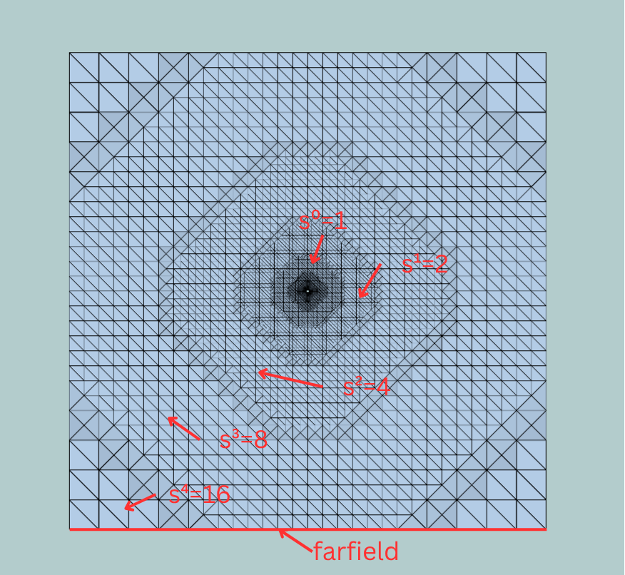
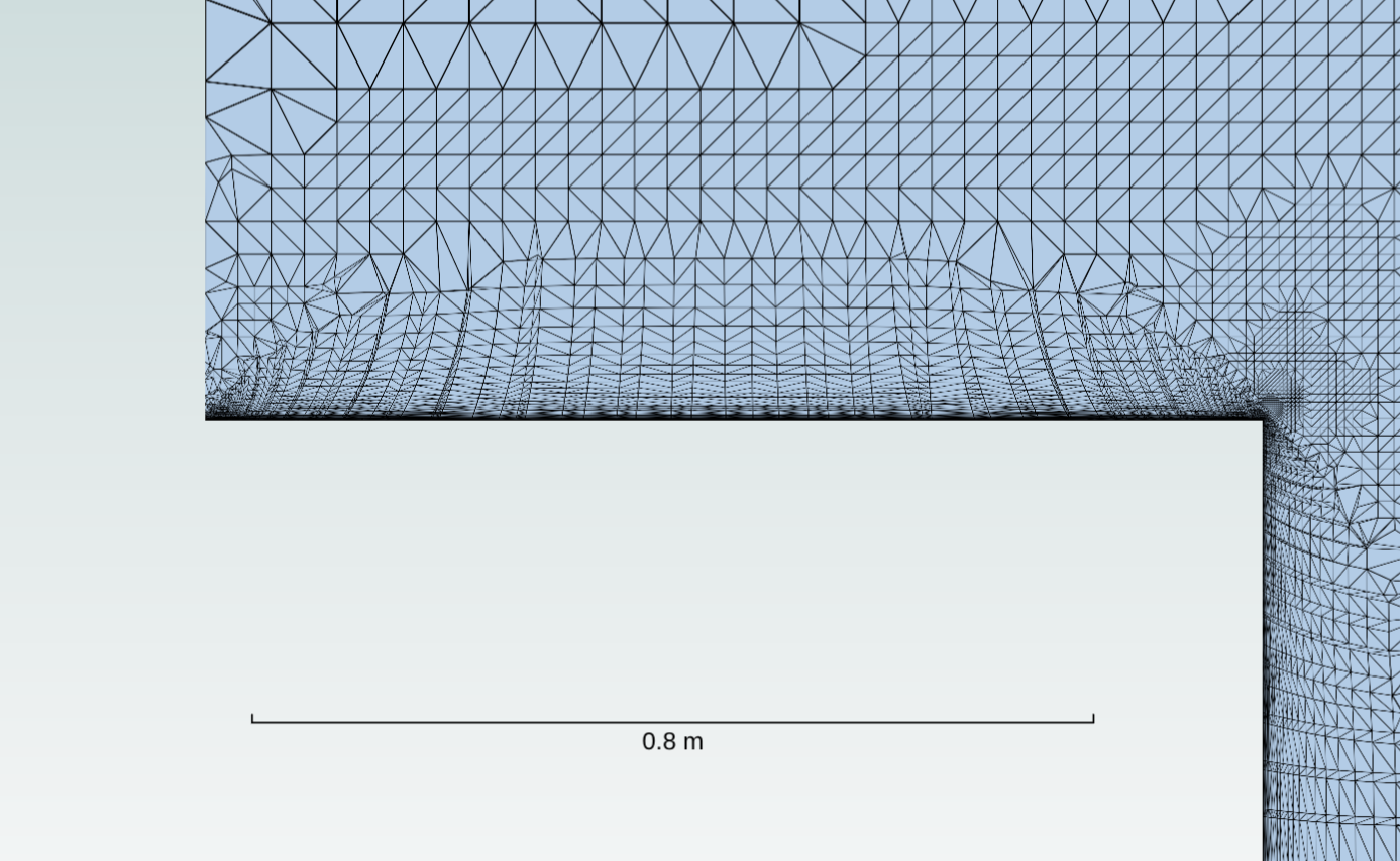
Farfield view: away from the geometry the octree coarsens, \(s_k = s_0 \cdot 2^{k}\) for \(k = 0 \dots 4\) (up to \(16\,s_0\)).# |
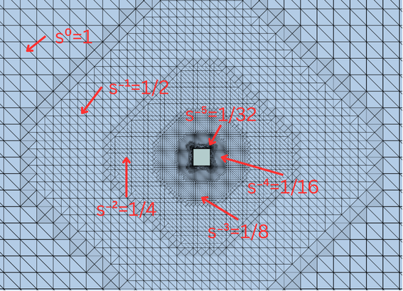
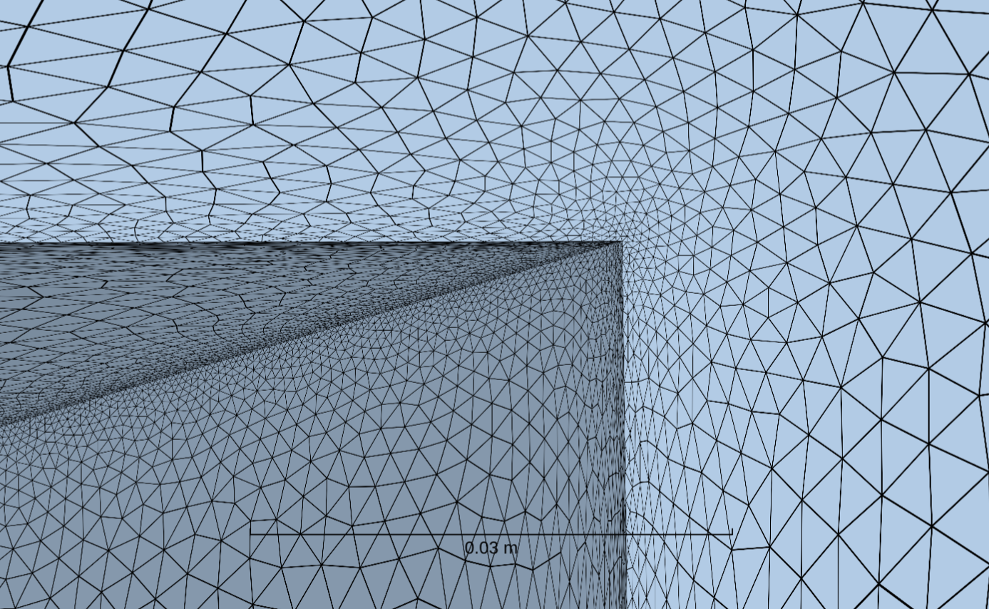
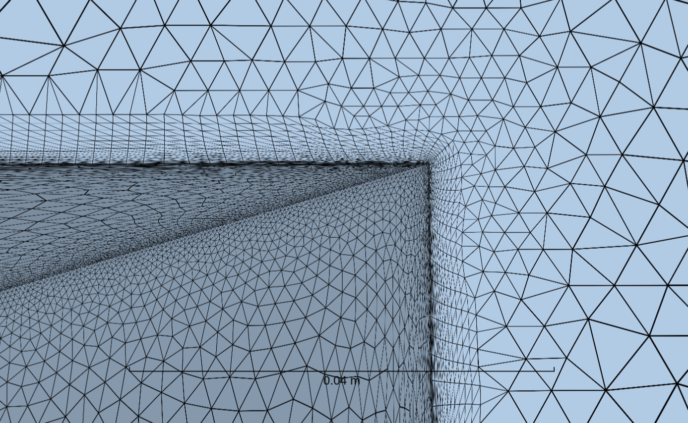
Zoom on the cube: toward the surface the octree refines, \(k = 0 \dots -5\) (down to \(s_0/32\)).# |
Slices through the farfield octree around a small cube at the centre, here with a base octree spacing of \(s_0 = 2\text{ m}\). Each level differs from its neighbour by a factor of two.
Note
The cells in these images appear to be tetrahedra, but this is mostly a visualisation artifact: the octree itself is made of hexahedral cells, which the visualisation pipeline triangulates for display. The exception is the transitions between refinement levels, which are genuinely meshed with tetrahedra to connect the differently-sized hexahedral regions.
A refinement spacing that does not exactly match a level in the series is cast to the first finer level (i.e. the next-smaller spacing), so the resulting mesh tends to be slightly finer than requested rather than coarser. A validation warning is emitted in that case so the rounding is visible.
How quickly the octree steps through these levels away from the surface is set by the volume edge growth rate (default 1.1, typical range 1.05–1.3, beta mesher only). The 2:1 ratio between neighbouring levels is fixed; this parameter instead controls how far apart the level transitions fall, and so how rapidly the mesh coarsens with distance from the geometry. Lower values keep the transitions closer together for smoother gradation at the cost of more cells, while higher values let the mesh coarsen faster with fewer cells. It is independent of the boundary layer growth rate, which governs the prism layers grown normal to the wall.
The base spacing can be overridden through the mesh parameters in the WebUI, or via the meshing defaults documented in the Python meshing API reference.
Custom volumes and zones#
By default, the Volume Mesher produces a single fluid zone. All enclosed regions are meshed as part of that single fluid zone; the mesher does not automatically exclude the interiors of nested bodies. To remove geometry that is not visible to flow (for example, a body nested inside another body), enable Remove hidden geometry; this option is available only with the GAI surface mesher.
How the farfield boundary is obtained depends on the farfield type: an automated farfield is generated automatically around the geometry, sized from its bounding box, whereas a user-defined farfield takes its boundaries from the supplied geometry file and meshes the region inside that geometry. Defining one or more custom volumes changes this: the mesher generates a separate volume zone for each custom volume in addition to the default fluid zone, so internal regions can carry their own mesh. On the solver side, custom zones default to fluid; mark a zone as solid to use it in a conjugate heat transfer simulation.
Two ways to define the geometry of a custom volume:
Enclosing-surface custom volume: list the surfaces whose closed shell bounds the region; each enclosing set produces one zone. Analytical primitives (cylinders, spheres, axisymmetric bodies) qualify as bounding entities only when they themselves define surfaces, which currently happens only for the interface of a rotation volume. Primitives that define refinement regions (axisymmetric or structured-box refinements) are volumetric regions of structured elements, not surfaces, and cannot be used to bound a custom volume.
Seedpoint volume: provide the coordinates of one or more interior seed points. The mesher runs a flood fill from those points to identify the zone, which is convenient for cavities bounded by many baffles. Available from release 25.10. Seedpoint volumes require the GAI surface mesher or snappy; they are not supported with the beta surface mesher or the legacy mesher. The number of seed points per volume differs by surface mesher: with the GAI surface mesher a seedpoint volume may carry several seed points, which the flood fill merges into one zone (useful when baffles split a single region into several compartments); with snappy each seedpoint volume must carry exactly one seed point.
Both definitions are wrapped in a custom zones container that lists which zones to generate and the element type to use inside them (mixed or tet-only). Bounding entities must not overlap between sibling custom volumes.
Note
When a custom volume encloses a rotating zone, its enclosing-surface list must include not only the custom volume’s own outer surfaces and the rotating zone’s sliding interface, but also every surface that lies inside that interface (for example, the rotor blades). The sliding interface resolves the patches it contains only when the parent custom volume lists them explicitly. For instance, a custom volume bounded by an outer surface that contains a sliding interface enclosing two bodies must list all of them together: the outer surface, the two enclosed bodies, and the interface.
Seedpoint volumes with the GAI surface mesher
With the GAI surface mesher, seedpoint volumes are supported as a single-zone workflow for setting up internal-flow cases. The simulation may define exactly one custom zones container, and that container may hold only seedpoint volumes (it cannot be combined with enclosing-surface custom volumes, nor with a second custom zones container). One or more seed points are flood-filled into that single internal zone. The snappy workflow does not have this restriction.
Rotating zones#
A rotating zone is a volume zone that participates in rotational motion at solver time (via the rotation model). Its sliding interface is meshed concentrically around the rotation axis, using three independent spacings: axial, radial, and circumferential. Rotating zones are built from a cylinder or axisymmetric body entity (the axisymmetric-body form needs the Volume Mesher). Donut shapes are supported: place a stationary centrebody (e.g. a hub) in the middle of the zone. A rotating zone can enclose other objects, but it cannot intersect them.
Important
The three spacings define the interface mesh only, not the interior of the zone. To control the mesh inside the zone, add a uniform refinement covering the rotating volume.
The rotating zone’s enclosed entities are the surfaces and nested regions sitting inside it (for example, rotor blades, a hub inside a donut zone, or a nested refinement region). Surfaces, cylinders, and axisymmetric bodies are always accepted; box and sphere enclosures require the Volume Mesher. In the Volume Mesher, surfaces among the enclosed entities can additionally be marked as stationary, indicating they are excluded from the rotation.
For spherical sliding interfaces, a separate rotation sphere zone type is available; it is built from a sphere entity and uses a single circumferential spacing.
Passive Spacings#
Passive spacing controls how the Volume Mesher treats the surface mesh on selected surfaces. Two types are available, each recommended for a different use case.
Unchanged
The unchanged passive spacing prevents the Volume Mesher from growing prism layers off the surface. Recommended for farfield surfaces, where boundary-layer resolution is not needed.
Note
Automatically generated farfield surfaces already use the unchanged passive spacing by default; you only need to set it explicitly on user-defined farfield surfaces.
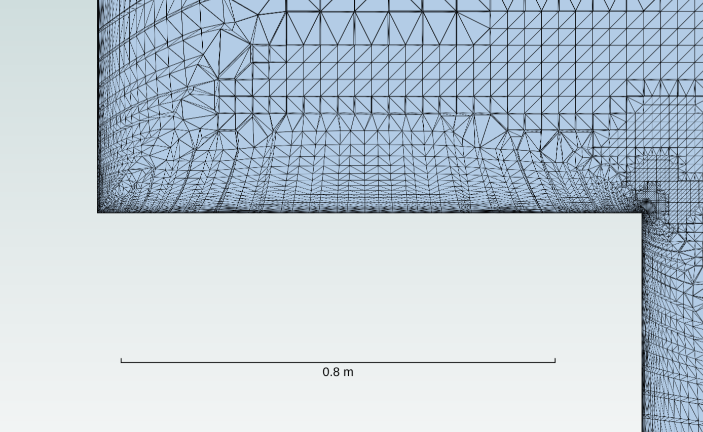
Default behaviour: prism layers are grown off the surface.# |
With unchanged passive spacing: no prism layers.# |
Projected
The projected passive spacing projects the neighbouring volumetric spacings onto the surface after the volume mesh has been generated, replacing the original surface mesh resolution on that surface. It can be applied to any planar surface (not only the symmetry plane) and to an axisymmetric sliding interface (a cylinder or axisymmetric body, but not an annular/donut cylinder). A free-floating sliding interface, and non-planar input surfaces, cannot be projected onto.
Examples#
Examples of mesh generation can be found in the Example Library. Specifically look at:
Isolated wing with BET Disk Model for Uniform and Axisymmetric refinements.
eVTOL Vehicle Mesh Generation for a rotating zone with interfaces.