3.2. Workflows & Interfaces

The workflows and interfaces section will explain the ways how the user can interact with Flow360 and go through the fundamental parts of performing the CFD simulation.

Interfaces

Flow360 allows the user to interact with the simulation and the data in two ways:

• through the web based WebUI,

• through the Python API.

Both interfaces allow users to set up cases, run simulations and manage their data and both of them rely on the same data, meaning that the case created through the Python API will be accessible and visible on the Web UI and vice versa.

Web UI

The WebUI provides a user with a graphical interface for the Flow360 solver. The WebUI offers a complete end-to-end CFD workflow in a cloud-based, browser-accessible environment.

Interface Specific Capabilities:

• Geometry Visualization & Inspection - Interactive 3D visualization of CAD geometry imported from multiple formats (STEP, IGES, SolidWorks, CATIA, etc.). Visual tools for inspecting geometric features including edges, faces, and bodies. Diagnostic tools for geometry quality assessment. Entity selection modes with visual highlighting. Boundary condition assignment with color-coded display. View controls including rotation, pan, zoom, and standard orientation presets via view cube.

• Mesh Visualization & Quality Analysis - Interactive 3D mesh inspection with configurable display modes (solid, wireframe, edges). Real-time visualization of mesh quality metrics including surface metrics (area, area ratio, aspect ratio, first layer height) and volume metrics (aspect ratio, volume). Element type statistics display (triangles, quads, tetrahedrons, prisms, pyramids, hexahedrons). Boundary layer visualization to verify thickness and growth rates. Length scale indicators for spatial reference.

• Comprehensive Simulation Setup - Define flow conditions, boundary conditions, 3D models (virtual propellers, BET disks, actuator disks), time stepping, and output settings. The built-in Inspector tool provides real-time validation with error detection.

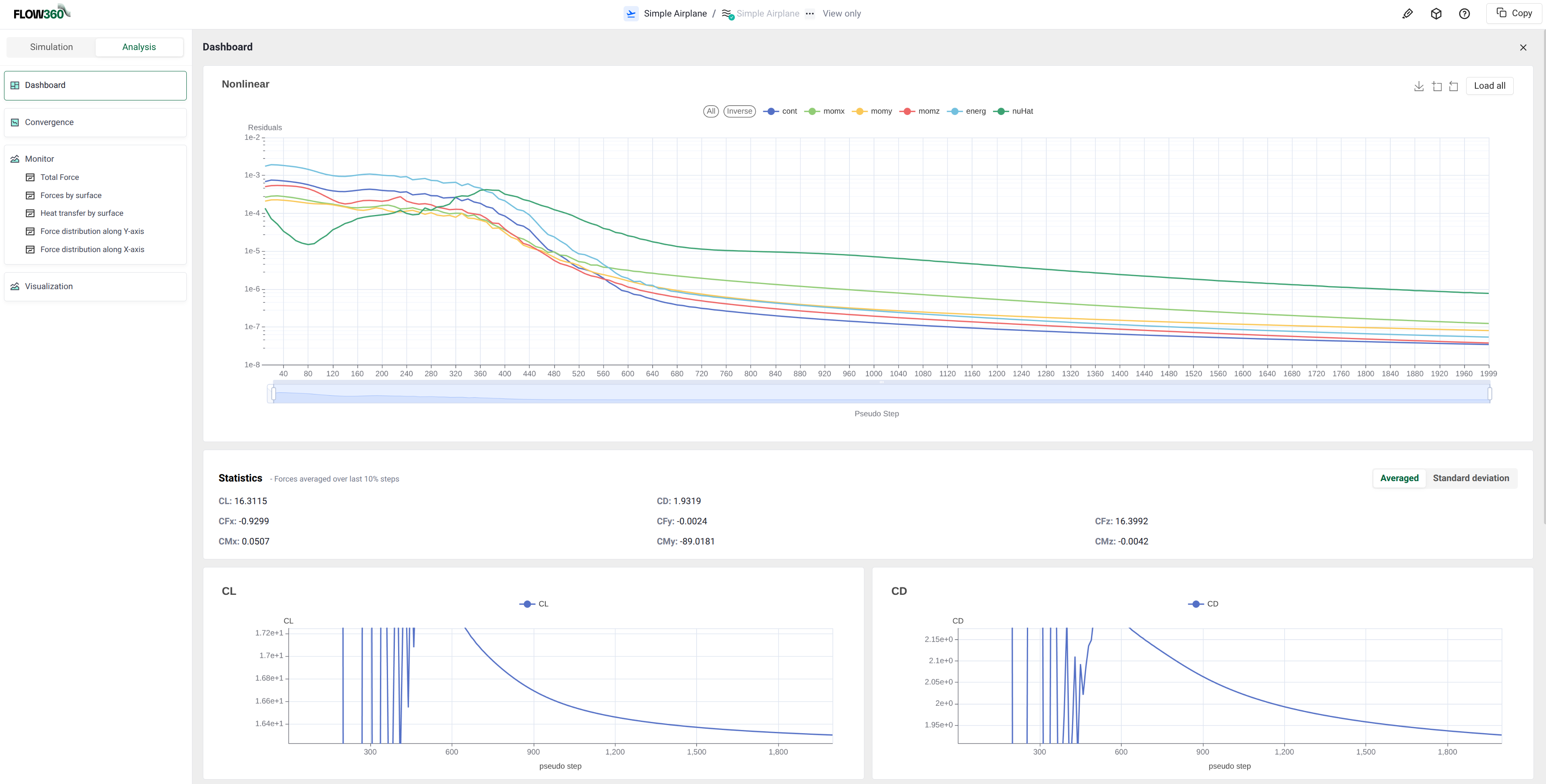
• Real-Time Monitoring - Track simulation progress with live residual plots, forces and moments (\(C_L\), \(C_D\), \(C_{Fx}\), \(C_{Fy}\), \(C_{Fz}\), \(C_{Mx}\), \(C_{My}\), \(C_{Mz}\)), convergence analysis, CFL evolution, and min/max flow variable monitoring. Specialized monitoring for heat transfer, BET analysis, and force distributions.

• Advanced Visualization - Four visualization modes: surface visualization (Cp, skin friction, y+), slice visualization (2D cross-sections), isosurface visualization (Q-criterion for vortex identification), and streamline visualization. Includes customizable colormaps with logarithmic/linear scaling.

• Case Comparison & Post-Processing - Compare multiple cases side-by-side, generate automatic result plots (e.g., CL vs alpha), create custom XY plots, and analyze convergence histories. Export results as CSV files and images.

The WebUI features a 7-panel workbench layout with an interactive 3D viewer, simulation setup panel, entities browser, navigation bar, status bar with Inspector tool, viewer mode controls, and persistent coordinate system reference.

The extensive guide for the Web UI can be found in the GUI Guide.

Python API

The Python API provides complete programmatic control of the Flow360 solver through the flow360 Python package. The API enables reproducible, scriptable CFD workflows with seamless integration into the Python scientific ecosystem, making it ideal for automation, parametric studies, and custom analysis pipelines.

Interface Specific Capabilities:

• Complete Workflow Automation - Programmatic control of the entire CFD workflow from geometry import through post-processing. Define meshing parameters, simulation setup, boundary conditions, time stepping, and output configurations entirely in Python scripts. Support for forking cases, mesh reuse optimization, and solution interpolation between meshes.

• Parametric Studies & Batch Processing - Run multiple cases in parallel on the cloud with simple loop structures. Automatic parallel execution for parameter sweeps (e.g., angle of attack, Mach number, design variables). Cases can be submitted simultaneously and monitored programmatically with case.wait() for efficient batch processing.

• Python Ecosystem Integration - Native integration with the scientific Python stack. Results automatically convert to Pandas DataFrames for data manipulation (results.total_forces.as_dataframe()). Seamless use of NumPy for calculations, Matplotlib for custom plotting, and SciPy for optimization. Full compatibility with machine learning libraries (TensorFlow, PyTorch) and optimization frameworks (PyOptSparse, Dakota) for design optimization workflows.

• Automated Report Generation - Generate PDF reports programmatically using the flow360.plugins.report module. Create customizable reports with 2D/3D charts, tables, convergence plots, and visualization snapshots. Apply statistical operations (averaging, min/max) to data items. Batch-generate reports across multiple cases for comparison studies.

The Python API unlocks powerful automation capabilities including design optimization loops, uncertainty quantification studies, machine learning model training, custom convergence criteria, real-time simulation control, and integration with external CAD/CAE tools. The combination of cloud-based parallel execution and Python’s rich ecosystem makes the API ideal for research applications, production workflows, and large-scale parameter explorations.

The documentation for the Python API can be found here with examples, reference or short snippets to help with commonly used operations.

Project Management

The Project

The basic container (environment) in Flow360 is a Project. The project is defined by its root asset which can be a geometry, a surface mesh and a volume mesh. The Project contains all the assets “derived” from its root and the user has access to every asset within.

Fig. 3.2.1 Project started from geometry

Fig. 3.2.2 Project started from surface mesh

Fig. 3.2.3 Project started from volume mesh

Dependent on the chosen type of root asset different file types are accepted:

• Geometry: ESP, EGADS, STEP, IGES, ACIS, AutoCAD-3D, Autodesk Inventor, CATIA V4-V6, Creo-Pro/E, I-deas, IFC, NX-Unigraphics, Parasolid, Revit, Rhino 3D, Solid Edge, SolidWorks, VDA-FS, UGrid, CGNS, STL

• Surface Mesh: UGrid, CGNS, STL (requires triangular elements)

• Volume Mesh: UGrid, CGNS (acceptable element types: tetrahedrons, hexahedrons, prisms, pyramids)

Important

When uploading a .lb8.ugrid file, to propagate the boundary names, the .mapbc file has to be in the same directory and has to have the same name.

Project Structure and Hierarchy

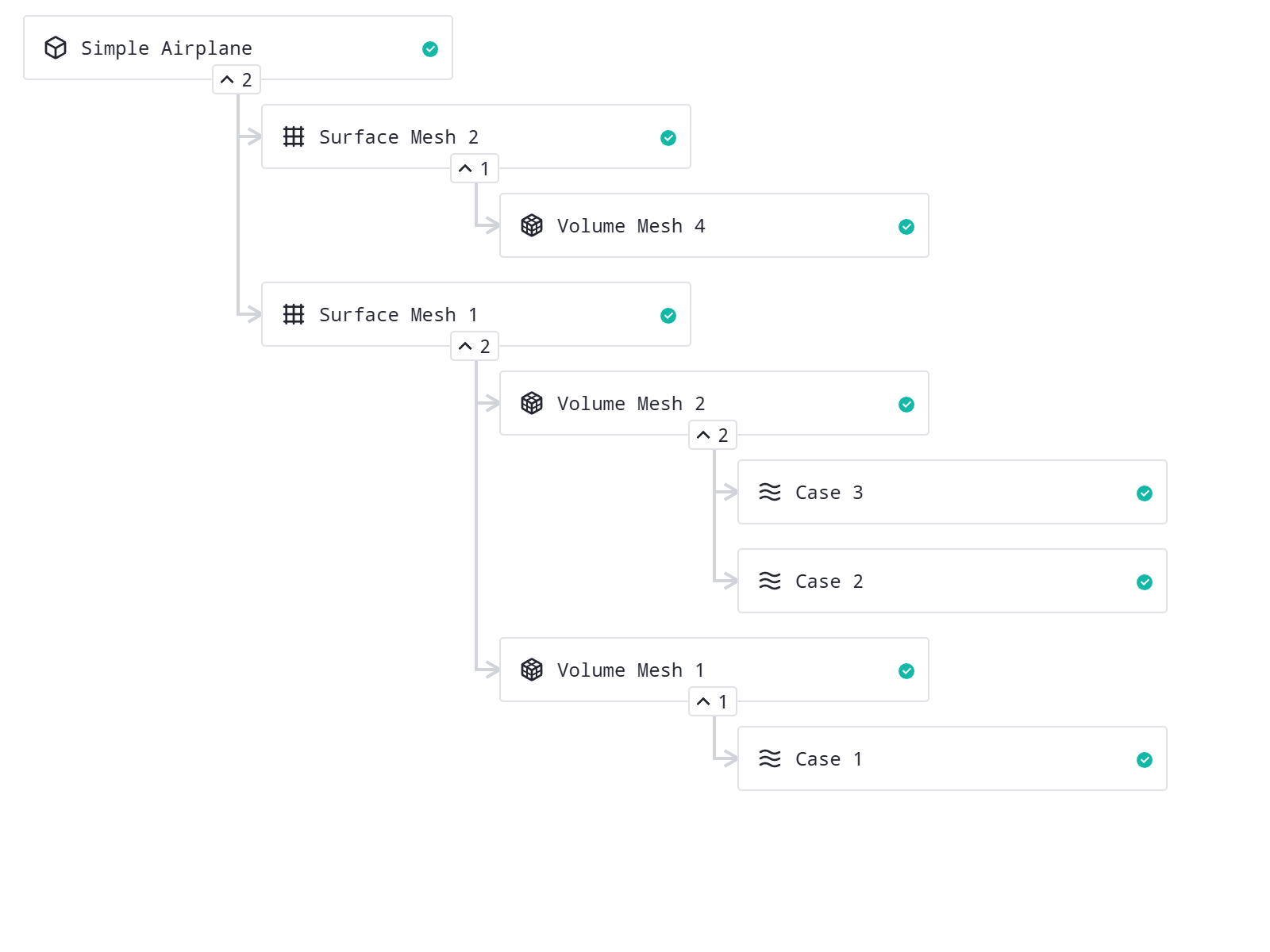
Flow360 organizes simulation resources in a flexible hierarchical structure that accommodates different workflow entry points and enables multiple analysis paths. The project structure follows a tree-like organization where each asset can branch into multiple downstream assets, supporting mesh sensitivity studies, parameter sweeps, and continuation runs.

In the WebUI, the project structure is visualized through the Project Tree, which displays the complete workflow of your CFD simulation from geometry to final results. The project tree is generated automatically based on your settings and intelligently identifies existing nodes that match your specifications. For example, if a surface mesh with identical settings already exists in the project, Flow360 will reuse it rather than generating a duplicate.

The workflow structure depends on the chosen entry point:

• Starting from geometry:

  Geometry
  └── Surface Mesh
      └── Volume Mesh
          └── Case
              └── Fork (optional)
  

• Starting from surface mesh:

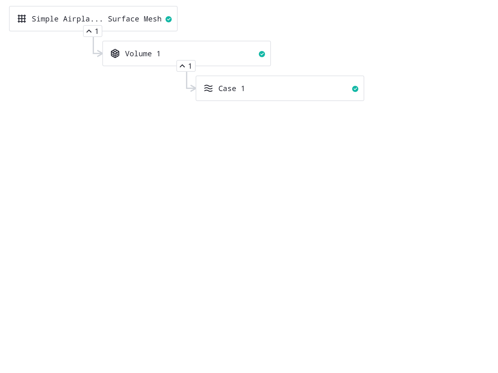
  Surface Mesh
  └── Volume Mesh
      └── Case
          └── Fork (optional)
  

• Starting from volume mesh:

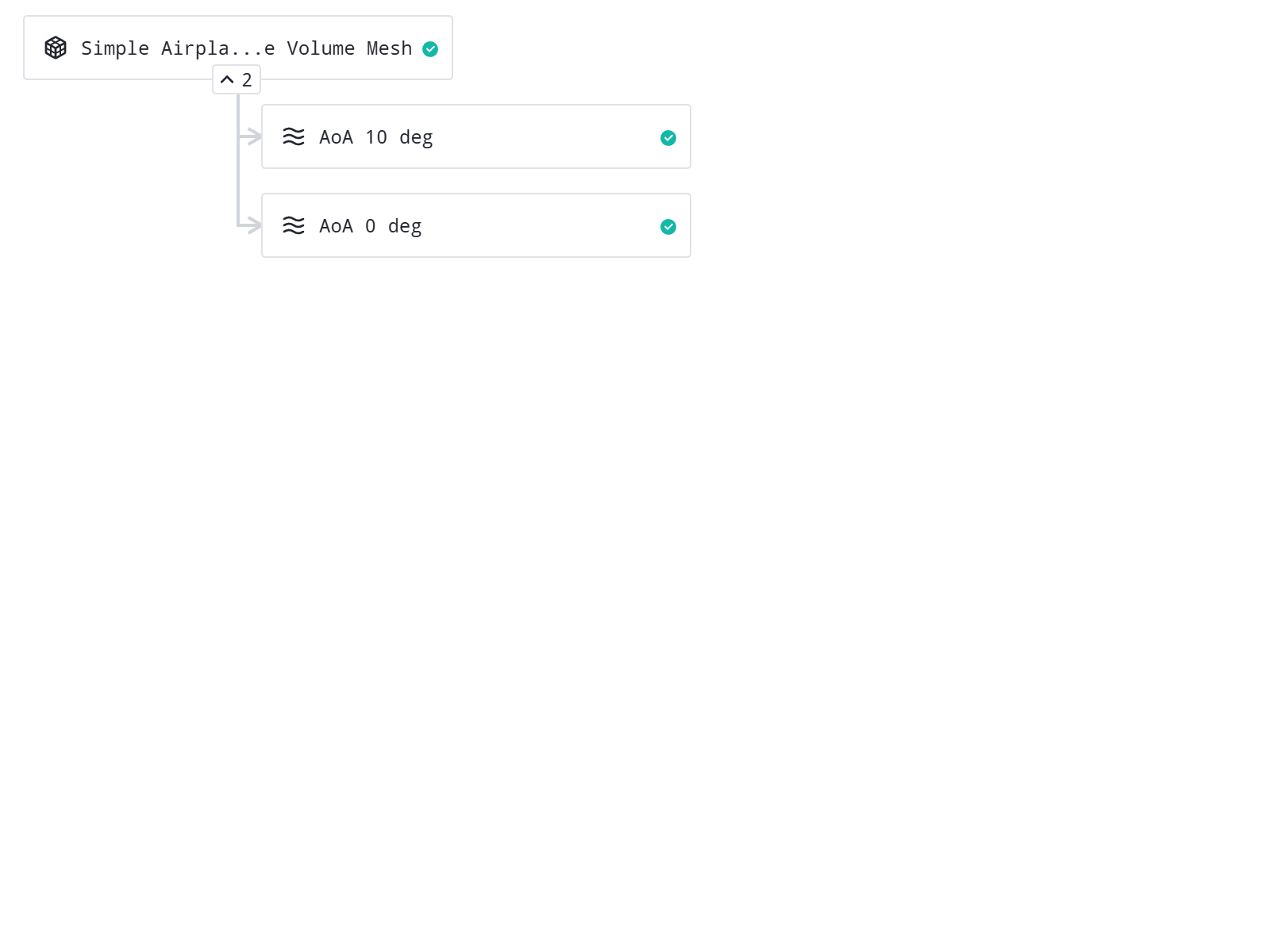
  Volume Mesh
  └── Case
      └── Fork (optional)
  

Each node in these hierarchies can branch into multiple parallel paths, enabling mesh sensitivity studies, parameter sweeps, and continuation runs from a single root asset.

For detailed visualization of the project tree and branching capabilities, see GUI Guide: Project Tree.

Asset Types

The following sections describe each cloud asset type available in Flow360. These assets form the hierarchical structure visible in the GUI Project Tree and can be created and managed through the Python API. In the WebUI, each asset type is represented by a distinct icon in the project tree.

Geometry

The Geometry asset represents the CAD geometry input for the simulation. The Geometry Python API class (see Cloud Assets) provides programmatic access to geometry asset properties and metadata, including face groups, edge groups, body groups, and other geometry attributes used for boundary condition assignment and meshing parameter configuration. For details on how face, edge, and body groupings work in the GUI, see GUI Guide: Geometry.

Geometry Requirements:

• For the legacy and new meshing workflows, it is required to have a clean, watertight geometry.

• For the GAI and snappy meshing workflow, it is not required to have a watertight clean geometry.

SurfaceMesh

The SurfaceMesh asset represents the discretized surface of the geometry, consisting of triangular elements that define the computational domain boundaries. Surface meshes are generated from geometry assets or can be uploaded directly as the project root asset.

In the project tree, surface meshes can branch into multiple volume meshes, each with different discretization parameters. This enables boundary layer resolution studies and mesh refinement analysis. Surface mesh quality metrics are available in the WebUI.

Surface Mesh Requirements:

• No self-intersections.

• All edges should be manifold (each edge shared by exactly two faces).

• Watertight surface mesh.

The SurfaceMesh Python API class (see Cloud Assets) provides access to surface mesh properties and metadata.

VolumeMesh

The VolumeMesh asset represents the complete 3D computational mesh used for simulation, containing tetrahedral, hexahedral, prismatic, or pyramidal volume elements. Volume meshes are generated from surface meshes or can be uploaded directly as the project root asset.

In the project tree, volume meshes can spawn multiple simulation cases, each with unique solver settings, facilitating parameter studies. An arrow on the volume mesh asset icon in the project tree indicates that the volume mesh exists in a different project, which is relevant for mesh interpolation workflows.

Volume Mesh Requirements:

• Watertight volume mesh.

• Positive volumes.

• Interfaces should be in contact with only two volume zones.

• The maximum distance between interfaces is 1 maximum edge length of the interface surfaces.

• Acceptable element types: tetrahedrons, hexahedrons, prisms, pyramids.

The VolumeMesh Python API class (see Cloud Assets) provides access to volume mesh properties and metadata. In the WebUI, volume mesh metadata including node counts, element statistics, and quality metrics can be viewed in the Entities Browser or by clicking the mesh metrics icon in the Viewer Region when in mesh view mode.

Case

The Case asset represents a simulation run with defined parameters, including meshing settings (when starting from geometry or surface mesh), operating conditions, boundary conditions, solver settings, and output configuration. Each unique combination of simulation parameters creates a separate case.

In the project tree, cases can be forked to create continuation runs. Forks are direct extensions of their parent cases, preserving all results and settings while allowing parameter modifications. Multiple forks can branch from the same parent case.

The Case Python API class (see Cloud Assets) provides programmatic control over case creation, parameter modification, submission, and result access.

Branching and Workflow Capabilities

The project structure supports multiple branches at each level, enabling flexible workflows:

• Geometry Level: Can generate multiple surface meshes with different discretization parameters, useful for mesh sensitivity studies.

• Surface Mesh Level: Multiple volume meshes possible from a single surface mesh, supporting different volume mesh parameters and enabling boundary layer resolution studies.

• Volume Mesh Level: Can spawn multiple simulation cases with unique solver settings, facilitating parameter studies.

• Case Level: Supports forking for continuation runs. Forks inherit all case results and settings while allowing parameter modifications.

For a visual guide to branching capabilities and project tree navigation, see GUI Guide: Project Tree.

Resource Reuse and Optimization

Flow360 automatically optimizes computational resources through intelligent asset reuse:

• Running standalone meshing: It is not mandatory to run all the parts of the simulation at once (surface meshing, volume meshing, case). The user can only choose to run up to the surface or volume mesh to examine its quality before launching a simulation.

Important

To continue the simulation from an already generated mesh, the parameters defining it must match exactly. Then the Reuse resource mechanism will make sure the mesh is not generated twice.

• Automatic Mesh Reuse: When submitting a new simulation, the system analyzes meshing parameters against existing meshes in the project tree. If an identical mesh configuration exists, that mesh is automatically reused rather than regenerating it. This eliminates redundant meshing operations when running parameter studies where only simulation conditions (e.g., angle of attack, Mach number) change while geometry and mesh settings remain constant.

Case Forking

Completed simulations can be forked to create continuation runs. Forking reuses the existing solution as an initial condition while allowing modification of any simulation parameters. This is particularly useful for extending convergence, performing parameter sweeps from a converged baseline, or adapting time step sizes. The forked case inherits the parent’s solution field while using the updated configuration.

Example usage of forking can be found in the Python API Example Library:

• Alpha sweep example

Results Interpolation

Solutions can be interpolated between different meshes of the same or similar geometry. This allows to reuse the results of one run as a starting point for another simulation.

Common use cases include:

• Using the results from a coarse mesh to initialize for a run on a denser mesh

• Forking the simulation to run with a slightly different geometry, such as different flap or radar angles

• Initializing the flow-field with a BET Disk simulation and then changing it to fully-resolved blade simulation for simulations that include rotors/propellers

Important

The case that will result from the interpolation will be a child case from which the results were taken to be interpolated.

Simulation Setup

Flow360 employs a unified configuration approach where preprocessing (meshing), simulation controls, and post-processing outputs are defined together in a single comprehensive setup. This “fire-and-forget” workflow enables users to configure the entire CFD process at once and submit it for asynchronous execution on the cloud, eliminating the need to manually manage workflow dependencies.

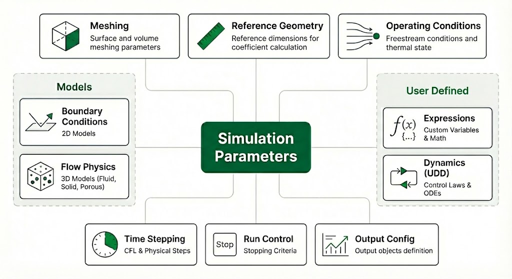
Fig. 3.2.4 Simulation parameters structure showing the unified configuration approach

The simulation configuration encompasses all aspects of the CFD workflow, organized into the following components:

• Meshing Parameters: Integrated within the same configuration, meshing parameters control automated mesh generation from geometry. Flow360 allows a couple of meshing workflows incluidng the legacy full meshing workflow and three surface meshers (GAI, Watertight Surface Mesher and snappyHex surface mesher) that work with the proprietary octree based Volume Mesher.

• Reference Geometry: Defines reference dimensions for non-dimensional coefficient calculations. This includes the moment reference center (the point about which moments are calculated), moment length dimensions (e.g., wingspan for \(C_{My}\), chord length for \(C_{Mx}\)), and the reference area (e.g., wing planform area) used for normalizing forces and moments. More about the non-dimensionalization can be found in the Non-Dimensionalization section.

• Operating Conditions: Specifies the freestream flow state for the simulation. For gas flows, users define either velocity magnitude or Mach number, along with angle of attack (\(\alpha\)) and sideslip angle (\(\beta\)). The thermal state can be specified using density and temperature, or by selecting standard atmosphere conditions. For liquid flows, velocity magnitude, density, and dynamic viscosity are required along with flow angles.

• Boundary Conditions: Assigns physical boundary types to geometric surfaces. Details about the Boundary conditions can be found under 2D models.

• Flow Physics: Is defined using a set of volumetric models that include the models that govern the material behaviour in the domain and introduce equations to be solved like the Fluid or Solid as well as reduced volumetric models like Porous media or BET disc that modify those equations in a specific volume to achieve the desired phenomena. The models responsible for equations also contain the settings for the solvers solving the introduced equations. The list of the models and their specifics can be found in 3D Models.

• Time Stepping: Controls temporal advancement of the solution. For steady-state simulations, users specify maximum pseudo-time iterations and CFL (Courant-Friedrichs-Lewy) number control strategy—either adaptive CFL with automatic adjustment based on convergence behavior, or ramped CFL with linear progression between initial and final values. For time-accurate (unsteady) simulations, physical time step size and number of steps are specified, along with maximum pseudo-iterations per physical time step and temporal order of accuracy (1st or 2nd order).

• Run control: Provides control over the stopping criteria of the simulation. Stopping criteria automatically terminate simulations when monitored output fields (force coefficients, probe values, or surface probe data) reach specified tolerance thresholds. See Run Control for detailed information.

• Output Configuration: Specifies post-processing data to be generated during the simulation. Users define volume outputs (3D flow field data throughout the domain), surface outputs (data on specified boundaries such as pressure coefficient, skin friction, heat transfer), slice outputs (2D cross-sectional views at specified planes), probe outputs (time-history data at point locations), isosurface outputs (surfaces of constant value like Q-criterion for vortex identification), aeroacoustic outputs (for noise prediction), force outputs (force and moment coefficients on specified models with optional moving statistics), and force distribution outputs (custom force and moment distributions along specified directions). Output fields include pressure coefficient, Mach number, velocity components, vorticity, Q-criterion, temperature, density, turbulence quantities, and many others. For time-accurate simulations, time-averaging outputs compute statistical quantities (mean, RMS) over specified time windows. For more information about available outputs see Output Configuration.

Additionally, the user can also specify their own flow variables, expressions, or user defined dynamics to control the solution:

• User Defined Expressions: Flow360 supports custom mathematical expressions through User Defined Expressions that enable advanced customization of simulation inputs and outputs. Users can define UserVariable objects that combine solution variables, geometry data, and mathematical operations using symbolic expressions. These custom variables can be used to compute derived quantities such as custom force components (e.g., hinge torques calculated from cross products of position vectors and surface forces), integrated values over surfaces or volumes, or specialized flow field quantities. User defined expressions support a comprehensive set of mathematical operations including arithmetic operators, trigonometric functions, vector operations (dot product, cross product, magnitude), conditionals, and spatial derivatives. These expressions can be referenced in output configurations to generate custom post-processing data tailored to specific analysis requirements.

• User Defined Dynamics: For advanced simulation control, Flow360 provides User Defined Dynamics (UDD) that allows users to implement custom time-dependent control laws and coupled physics. UDD enables definition of auxiliary state variables governed by ordinary differential equations (ODEs) that evolve during the simulation. These state variables can depend on flow solution quantities (forces, moments, pressures at specific locations) and can be used to control boundary conditions or body motions in real-time. Common applications include flight dynamics coupling (where aircraft motion responds to aerodynamic forces), active flow control (where actuators respond to flow sensors), aeroelastic coupling with simplified structural models, and closed-loop control systems (such as angle of attack controllers maintaining target lift coefficients). The ODE systems are integrated alongside the flow equations, enabling fully coupled multiphysics simulations. UDD state variables can be monitored as outputs and used in user defined expressions for post-processing.

Results Processing

The results from Flow360 are stored as a case asset. These results can be downloaded and processed using the Python API or the WebUI. The results are defined from the output list specified in the simulation setup. In general two types of results are generated:

Tabulated Data

This includes all data that is sampled per time step or iteration like the CFL number, residuals, forces, moments, heat transfer, monitors, etc. This data is usually plotted as a function of time or iteration. The data is stored in CSV files. The processing of this data is already done automatically in webUI, if user wants to download the data and process it manually, the data can be downloaded from the Assets button or using the Python API.

By default, Flow360 creates the following results files:

• Case configuration (inputs): The full set of inputs used to run the case are in simulation.json, which define the physics models, boundary conditions, numerics, and requested outputs.

• Run logs: Human-readable logs that capture the run history, warnings, and solver messages are in logs/flow360_case.user.log.

• CFL history: CFL history over iterations/time is in results/cfl_v2.csv.

• Residual histories: Convergence histories for the linear and nonlinear solves are in results/linear_residual_v2.csv and results/nonlinear_residual_v2.csv.

• Max-residual location: The spatial location (and associated metadata) of the maximum residual for debugging convergence issues are in results/max_residual_location_v2.csv.

• Min/Max state monitoring: Min/max tracked solution-state quantities over the run with the location of the minimum and maximum values are written in results/minmax_state_v2.csv.

• Integrated forces and moments: Case-level totals of forces/moments (and coefficients, depending on setup) over the run are in results/total_forces_v2.csv.

• Surface forces: Per-surface integrated forces/moments broken down by boundary/surface group are in results/surface_forces_v2.csv.

• Surface heat transfer: Per-surface integrated heat-transfer quantities are in results/surface_heat_transfer_v2.csv.

• Slice force distributions: Force distributions along specified slicing directions are in results/X_slicing_forceDistribution.csv and results/Y_slicing_forceDistribution.csv.

Tip

The tabular data can be easily processed with the use of the Python API through the case.results objects that also provide useful processing functions like averaging or sorting by entity.

See also

• Forces and Moments dimensionalization guide

• Forces and Moments dimensionalization snippet

Spatial Data

Spatial data contains flow variables available on the computational mesh. The available types of spatial data are:

• Surface data: data on the surface mesh

• Volume data: data in the volume mesh

• Slice data: data on the slice planes

• Isosurface data: data on the isosurfaces, ant the isosurfaces themselves

• Streamlines

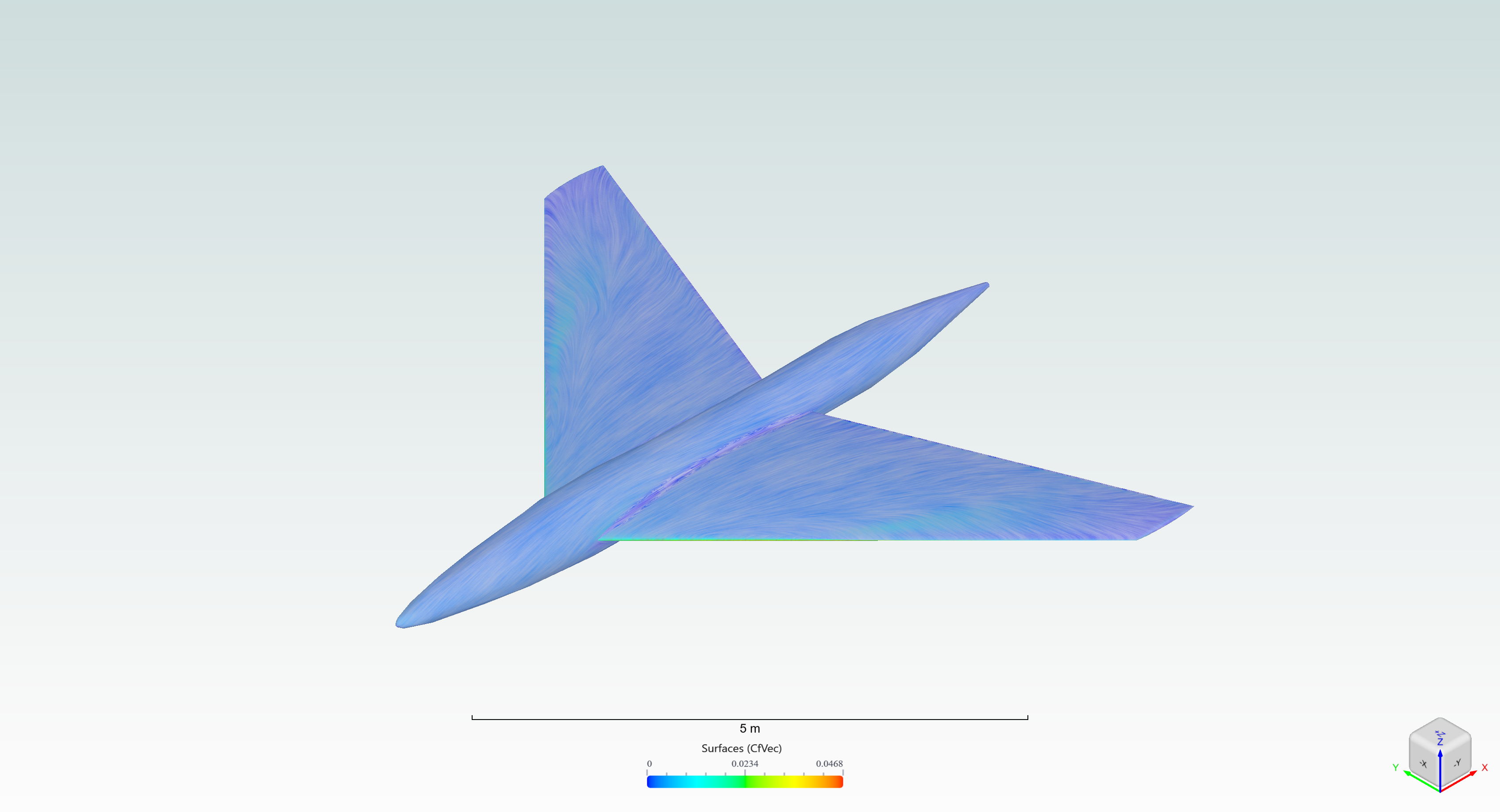
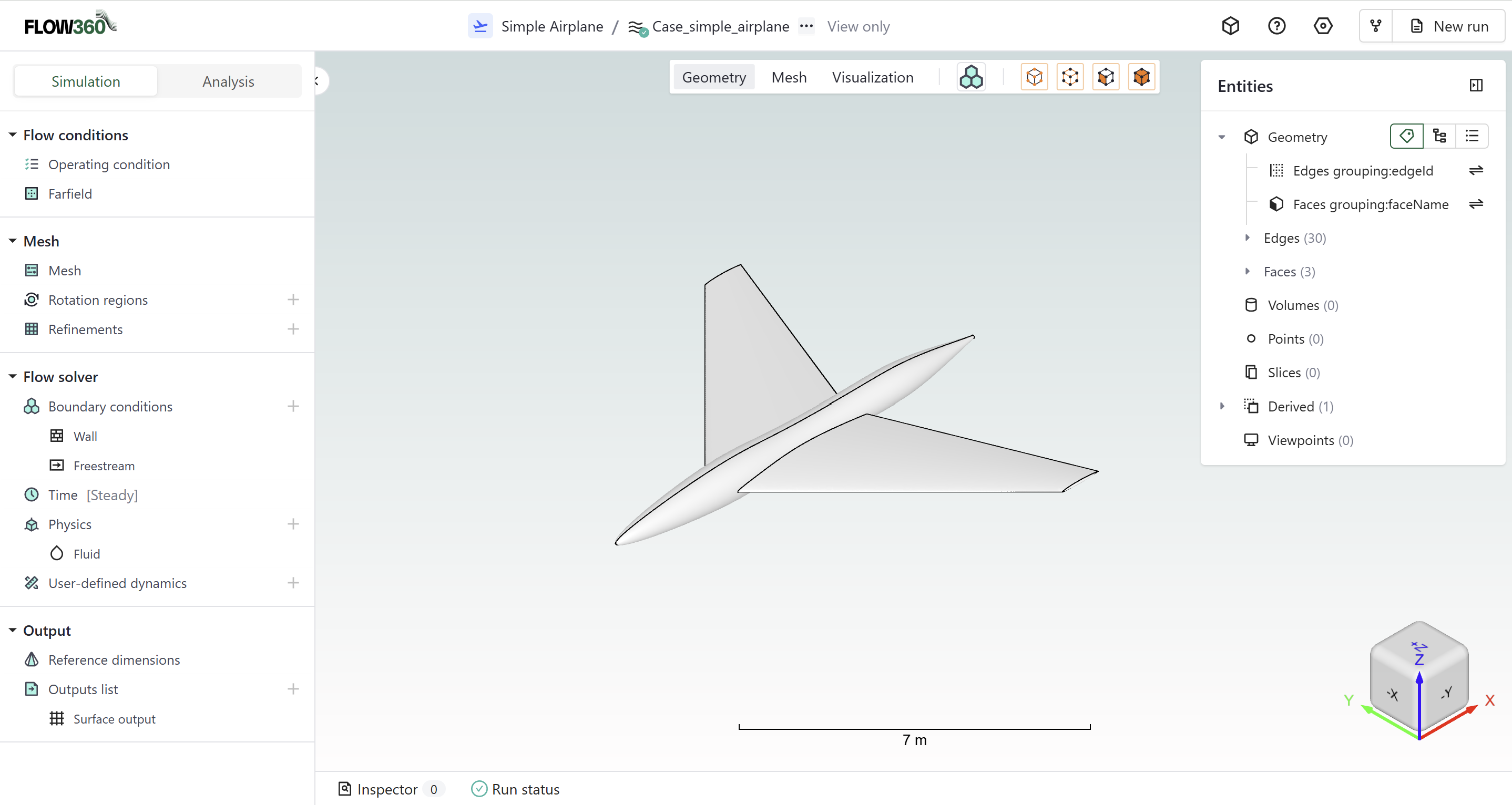
Fig. 3.2.5 Example CfVec contour on a Simple Airplane geometry, visualised in Web UI.

By default, Flow360 creates the following:

• Surface: Data on the wall boundaries, with variables: Cf, CfVec, yPlus, Cp, forcesPerUnitArea, heatFlux, nodeNormals, T.

• Slices: Data on the main slice planes (XY, XZ, YZ), going through the mesh origin, with variables: primitiveVars, T.

• Isosurface: qCriterion isosurface with a Mach variable.

Spatial data can be visualised directly in webUI by going to the Analysis tab and selecting the Visualization section.

Tip

If user wants to download the data and process it manually, the data can be downloaded from the Assets button or using the Python API. Open the data in ParaView, Tecplot or any other supported software. The relevant files for each output can be found in the Available Outputs section.

Related Topics

• User Guide: Meshing - Detailed information on surface and volume mesh generation

• Cloud Assets API Reference - Python API classes for Project, Geometry, SurfaceMesh, VolumeMesh, and Case

• GUI Guide: Project Tree - Project structure visualization and navigation in the WebUI

• GUI Guide: Starting a Project - Creating projects from geometry, surface mesh, or volume mesh