Report

3.11. Report#

This section describes how to use the automatic reporting plugin for Flow360 simulations to generate professional PDF reports from your simulation results.

Important

The report functionality is currently available only through the Python API.

Overview#

The report plugin:

Loads simulation data from one or more Case objects.
Extracts relevant metrics, such as velocities, forces, boundaries, and other fields.
Creates custom sections (e.g. Summary, Inputs, Tables, Charts) and assembles them into a single LaTeX-based PDF document.
Can create plots of force convergence or dependencies of result variables on input parameters for multiple cases (for example, CL vs alpha, CD vs Re, etc.).
Can optionally include 3D images or screenshots of the geometry, surfaces, or isosurfaces for an at-a-glance view of simulation geometry or results.

Constructing a report template#

A report is constructed using the ReportTemplate class. You define a list of report items (such as summaries, tables, and charts) that will be assembled into the final PDF document.

Basic structure:

from flow360.plugins.report import ReportTemplate
from flow360.plugins.report import Summary, Inputs, Table, Chart2D

report = ReportTemplate(
    title="Aerodynamic analysis of DrivAer",
    items=[
        Summary(text="This report summarizes the CFD analysis results."),
        Inputs(),
        Table(
            data=[
                "params/reference_geometry/area",
                "params/time_stepping/max_steps",
            ],
            section_title="Simulation Parameters",
        ),
        Chart2D(
            x="surface_forces/pseudo_step",
            y="surface_forces/totalCD",
            section_title="Drag Coefficient Convergence",
            fig_name="cd_convergence",
        )
    ]
)

Creating reports in the cloud:

# Submit report generation to the cloud
import flow360 as fl

cases = [fl.Case.from_cloud("case_id_1"), fl.Case.from_cloud("case_id_2"), fl.Case.from_cloud("case_id_3")]

report_job = report.create_in_cloud(
    name="My Report",
    cases=cases
)

# Wait and download
report_job.wait()
report_job.download("report.pdf")

Saving and loading report templates:

Report templates can be saved to JSON files for reuse:

# Save template to JSON
report.to_file("report_template.json")

# Load template from JSON
report = ReportTemplate(filename="report_template.json")

How to access the simulation data#

Data paths are specified as strings that navigate through the case’s data structure. The path components are separated by / and correspond to nested attributes, dictionary keys, indices or functions that can be called on the data. The results attribute does not have to be specified to access the data, it is automatically added to the path.

Example data paths:

Simulation parameters: params/operating_condition/velocity_magnitude, params/time_stepping/max_steps
Reference geometry: params/reference_geometry/area, params/reference_geometry/moment_length/0
Surface forces: surface_forces/totalCD, surface_forces/totalCL, surface_forces/totalCMz
Total forces: total_forces/CL, total_forces/CD
Residuals: nonlinear_residuals/pseudo_step, nonlinear_residuals/0_cont
Mesh information: volume_mesh/stats/n_nodes, volume_mesh/bounding_box/length

Using DataItem for advanced data access:

The DataItem class provides more control over data retrieval, including operations like averaging and filtering by boundary:

from flow360.plugins.report import DataItem, Average

# Average the last 10% of data
DataItem(
    data="surface_forces/totalCD",
    operations=[Average(fraction=0.1)]
)

# Include only specific boundaries
DataItem(
    data="surface_forces/totalCD",
    include=["body", "wing"]
)

# Exclude boundaries from calculation
DataItem(
    data="surface_forces/totalCD",
    exclude=["farfield"]
)

Recommended

It is recommended to use the DataItem class to access the data, as it provides more control over the data retrieval and processing.

`Case` object selection#

The cases for which the report is generated should be specified using the cases argument of the create_in_cloud() method. When working with multiple cases, you can control which cases are included in specific report items:

select_indices: Specify which cases (by index) to include in a chart or table.
separate_plots: When True, creates individual plots for each case.
group_by: Group cases by a specific parameter for comparison plots.

Chart2D(
    x="params/operating_condition/alpha",
    y=DataItem(data="surface_forces/totalCL", operations=[Average(fraction=0.1)]),
    section_title="CL vs Alpha",
    fig_name="cl_alpha",
    select_indices=[0, 1, 2],  # Only include first three cases
    separate_plots=False,      # Overlay all cases on one plot
)

Tables (`Table`)#

Tables display simulation data in a structured format. Each row represents a case, and each column represents a data field.

Basic table example:

Table(
    data=[
        "params/reference_geometry/area",
        "params/operating_condition/velocity_magnitude",
        DataItem(data="surface_forces/totalCD", operations=[Average(fraction=0.1)]),
    ],
    section_title="Results Summary",
    headers=["Reference Area", "Velocity", "Avg. CD"],
)

Table options:

data: List of data paths or DataItem objects to display as columns.
section_title: Title displayed above the table.
headers: Custom column headers (must match length of data).
formatter: Format specifier for numeric values (e.g., ".4g" or a list of formatters).
select_indices: Include only specific cases by index.

Graphs (`Chart2D`)#

2D charts visualize relationships between data variables across one or more simulation cases.

Basic chart example:

Chart2D(
    x="surface_forces/pseudo_step",
    y="surface_forces/totalCD",
    section_title="Drag Coefficient",
    fig_name="cd_plot",
)

Chart options:

x: Data path for the x-axis.
y: Data path for the y-axis (can be a list for multiple series).
section_title: Title displayed above the chart.
fig_name: Unique identifier for the figure file.
fig_size: Relative size of the figure (default: 0.7).
y_log: Set to True for logarithmic y-axis scale.
show_grid: Display grid lines (default: True).

Time series based and case based data#

Charts can display two types of data:

Time series data (e.g., convergence history):

# Each case contributes a line showing evolution over time/steps
Chart2D(
    x="surface_forces/pseudo_step",
    y="surface_forces/totalCD",
    section_title="CD Convergence History",
    fig_name="cd_history",
)

Case-based data (e.g., parameter sweeps):

# Each case contributes a single point (e.g., averaged value)
Chart2D(
    x="params/operating_condition/alpha",
    y=DataItem(data="surface_forces/totalCL", operations=[Average(fraction=0.1)]),
    section_title="CL vs Alpha",
    fig_name="cl_alpha",
)

Important

It is important to make sure that the data retrieved for the x and y axes has the same length.

Time and pseudo step domain#

For unsteady simulations, you can plot against either pseudo steps or physical time:

# Plot against pseudo steps
Chart2D(
    x="surface_forces/pseudo_step",
    y="surface_forces/totalCD",
    ...
)

# Plot against physical time
Chart2D(
    x="surface_forces/time",
    y="surface_forces/totalCD",
    ...
)

The plugin automatically handles pseudo step accumulation across physical time steps for unsteady simulations.

Tip

When plotting against pseudo_step, when the number of physical steps visible within x axis limits is less or equal than 5, the secondary x axis with time will be shown.

Data grouping#

Use the group_by parameter to organize case-based data into groups for comparison:

from flow360.plugins.report import Grouper

Chart2D(
    x="params/operating_condition/alpha",
    y=DataItem(data="surface_forces/totalCL", operations=[Average(fraction=0.1)]),
    section_title="CL vs Alpha by Turbulence Model",
    fig_name="cl_alpha_grouped",
    group_by=Grouper(group_by="params/models/Fluid/turbulence_model_solver/type_name"),
)

This creates separate line series for each unique value of the grouping parameter.

Grouping with buckets:

When you want to combine multiple values into named groups, use the buckets parameter. This is useful when you have many cases with different tags or attributes that should be grouped together:

from flow360.plugins.report import Grouper

# Group cases by turbulence model AND by case tags
# Tags "baseline" and "reference" go into "Baseline" bucket
# Tags "optimized_v1" and "optimized_v2" go into "Optimized" bucket
Chart2D(
    x="params/operating_condition/alpha",
    y=DataItem(data="surface_forces/totalCL", operations=[Average(fraction=0.1)]),
    section_title="CL vs Alpha - Baseline vs Optimized",
    fig_name="cl_comparison",
    group_by=Grouper(
        group_by=[
            "params/models/Fluid/turbulence_model_solver/type_name",
            "info/tags/0"
        ],
        buckets=[
            None,  # Each turbulence model gets its own series
            {"Baseline": ["baseline", "reference"], "Optimized": ["optimized_v1", "optimized_v2"]}
        ],
    ),
)

In this example:

The first grouping level (turbulence_model_solver/type_name) has buckets=None, meaning each unique turbulence model creates a separate series.
The second grouping level (info/tags/0) uses buckets to combine multiple tag values into named groups.
The result is a chart with series like “kOmegaSST - Baseline”, “kOmegaSST - Optimized”, “SpalartAllmaras - Baseline”, etc.

Visualisations (`Chart3D`)#

3D charts generate screenshots of your simulation geometry or field results. These are rendered using an external visualization service and embedded into the PDF report.

Basic 3D visualization:

from flow360.plugins.report.report_items import Chart3D
from flow360.plugins.report.uvf_shutter import Camera

Chart3D(
    show="boundaries",
    field="Cp",
    limits=(-1.0, 1.0),
    camera=Camera(position=(-1, -1, 1)),
    section_title="Pressure Distribution",
    fig_name="cp_surface",
)

Chart3D options:

show: Type of object to display ("boundaries", "slices", "qcriterion", "isosurface").
field: Surface field to display (e.g., "Cp", "yPlus", "Cf").
limits: Min/max values for the field colormap.
is_log_scale: Use logarithmic colormap scaling.
camera: Camera configuration for the view.
include/exclude: Filter which boundaries to show.
mode: Display mode ("contour" or "lic" for line integral convolution).

Camera controls#

The Camera class controls the viewpoint for 3D visualizations. All length values are in the same units used in your geometry or volume mesh.

Key camera attributes:

position: The camera’s eye position in 3D space. Think of it as a point on a sphere looking inward toward look_at.
up: Vector determining which direction is “up” in the final image.
look_at: The target point the camera is aimed at. Defaults to the bounding box center.
pan_target: Point to pan the viewport center to (if different from look_at).
dimension: Controls zoom level - the rendered view will show this many model units.
dimension_dir: Direction for the dimension parameter ("width", "height", or "diagonal").

Camera example:

from flow360.plugins.report import Camera

# Custom camera view
Camera(
    position=(0, -1, 0),       # View from negative Y axis
    up=(0, 0, 1),              # Z-up orientation
    look_at=(0, 0, 0),         # Look at origin
    dimension=2.0,             # Show 2 model units width
    dimension_dir="width",
)

Preset cameras:

Several preset camera positions are available for convenience:

TopCamera: Looking down from above (+Z)
BottomCamera: Looking up from below (-Z)
FrontCamera: Looking from +X toward origin
RearCamera: Looking from -X toward origin
LeftCamera: Looking from +Y toward origin
FrontLeftTopCamera: Diagonal view from front-left-top
RearRightBottomCamera: Diagonal view from rear-right-bottom

Camera examples#

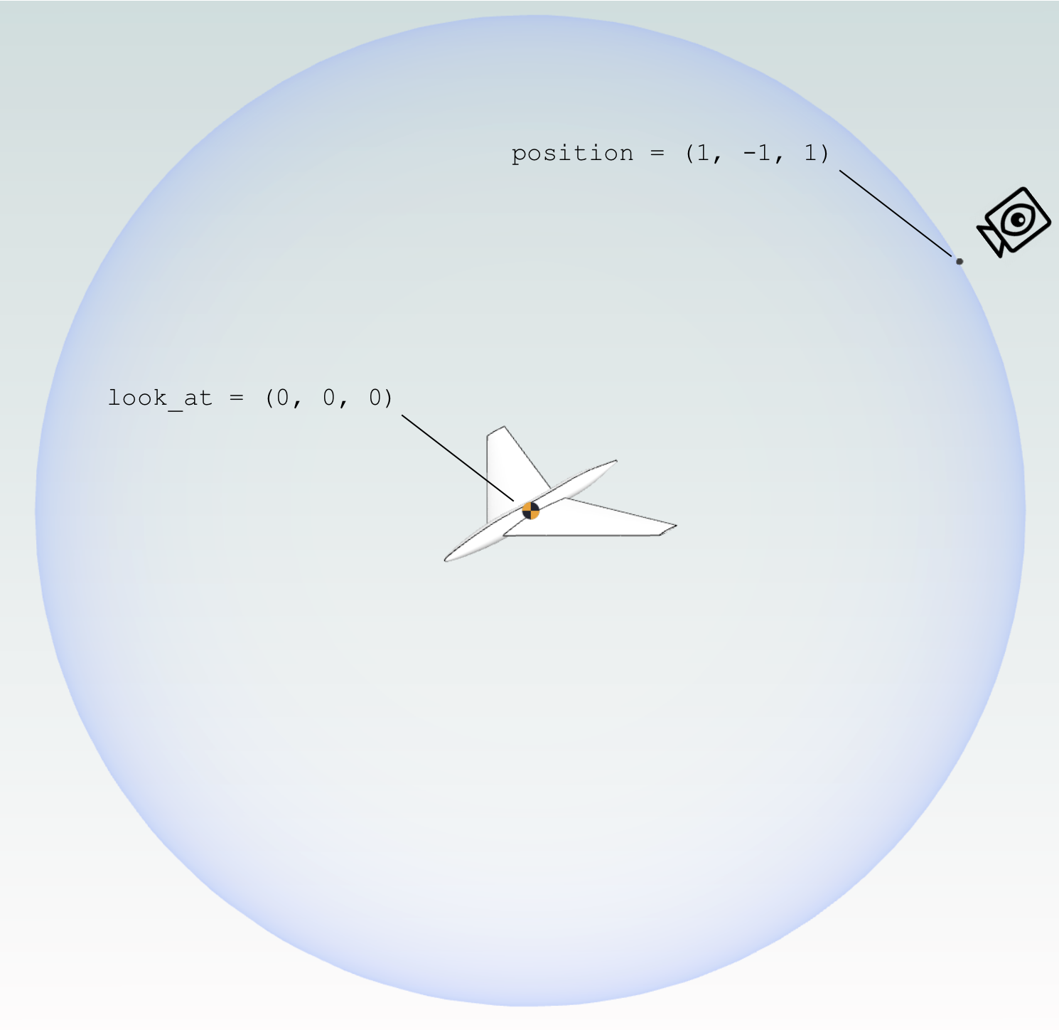
See how changing position and look_at affects the orientation of the camera.

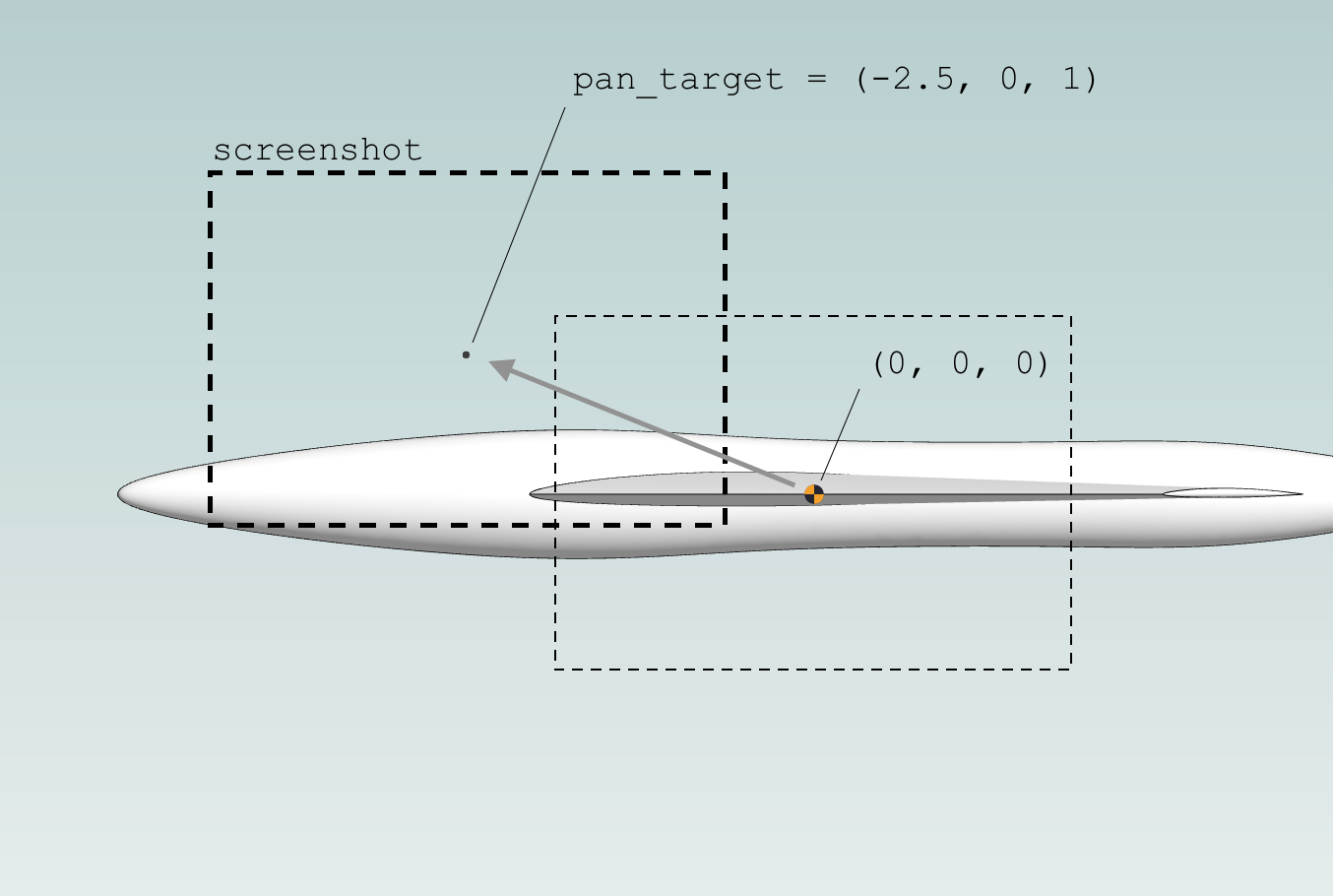
See how pan_target changes the view.

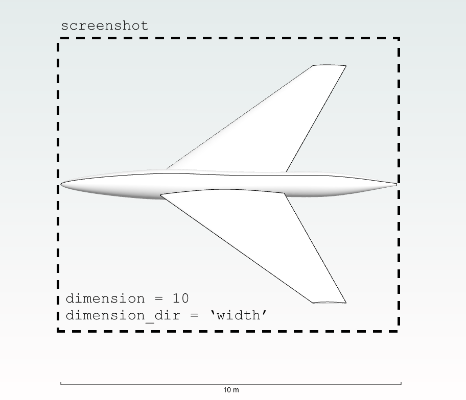
Camera dimension and dimension_dir example

See the effect of dimension and dimension_dir on zoom level.

Pre-prepared generic items#

The report plugin includes several pre-configured report items for common use cases.

`Summary`#

Adds a summary section at the beginning of the report with optional text and a table of case names and IDs.

Summary(
    text="This report presents the aerodynamic analysis results for the DrivAer model. "
         "Multiple configurations were tested at various operating conditions."
)

`Inputs`#

Automatically generates a table of key simulation input parameters extracted from the case configuration.

Inputs()

This will include: - Velocity magnitude - Time stepping type

`NonlinearResiduals`#

Generates a chart showing the convergence history of nonlinear residuals. This is a specialized version of Chart2D pre-configured for residual plotting with logarithmic y-axis.

NonlinearResiduals()

This automatically plots all residual components (continuity, momentum, energy, etc.) with appropriate formatting for convergence analysis.

Examples#

To see examples of how to use the report plugin, please refer to the Example Library. Specifically: