How Does It Work?#
Flow360 is a Cloud-Native Solver designed to decouple simulation setup from simulation execution.
Unlike traditional desktop CFD where you must keep your application open while the solver runs, Flow360 operates asynchronously. You define your simulation requirements, submit them to our cloud, and the system handles the rest automatically.
The Architecture (Client vs. Cloud)#
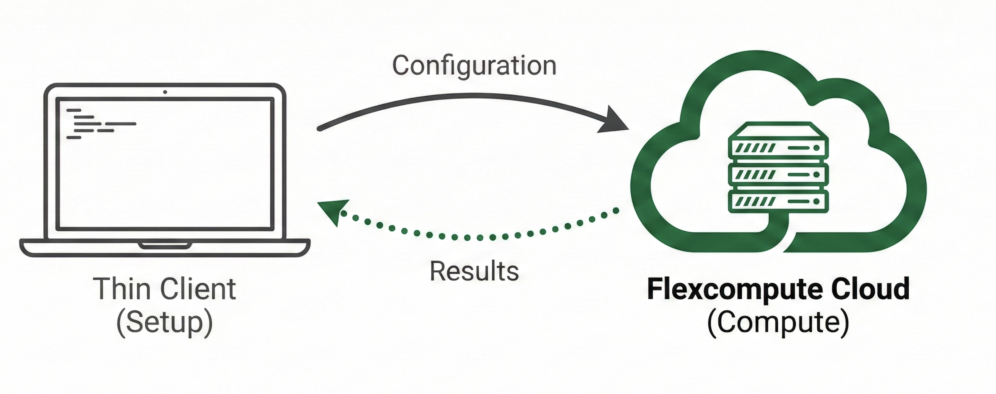
Flow360 operates on a Thin Client / Heavy Server model.
The Client (You): Your local environment is used only to define the simulation. You do this via the WebUI (browser-based forms) or the Python API (Python objects). No heavy computation happens on your machine.
The Cloud (Us): When you submit a case, your configuration is sent to the Flexcompute cloud. Our system provisions the necessary high-performance hardware (GPUs) to mesh, solve, and post-process your case.
Note
Connectivity: A standard internet connection is sufficient to configure and run simulations. High-bandwidth connections are only advantageous when interacting with large 3D visualization objects or downloading massive volume field datasets.
Automatic Orchestration (Fire and Forget)#
A key feature of Flow360 is Asynchronous Execution.
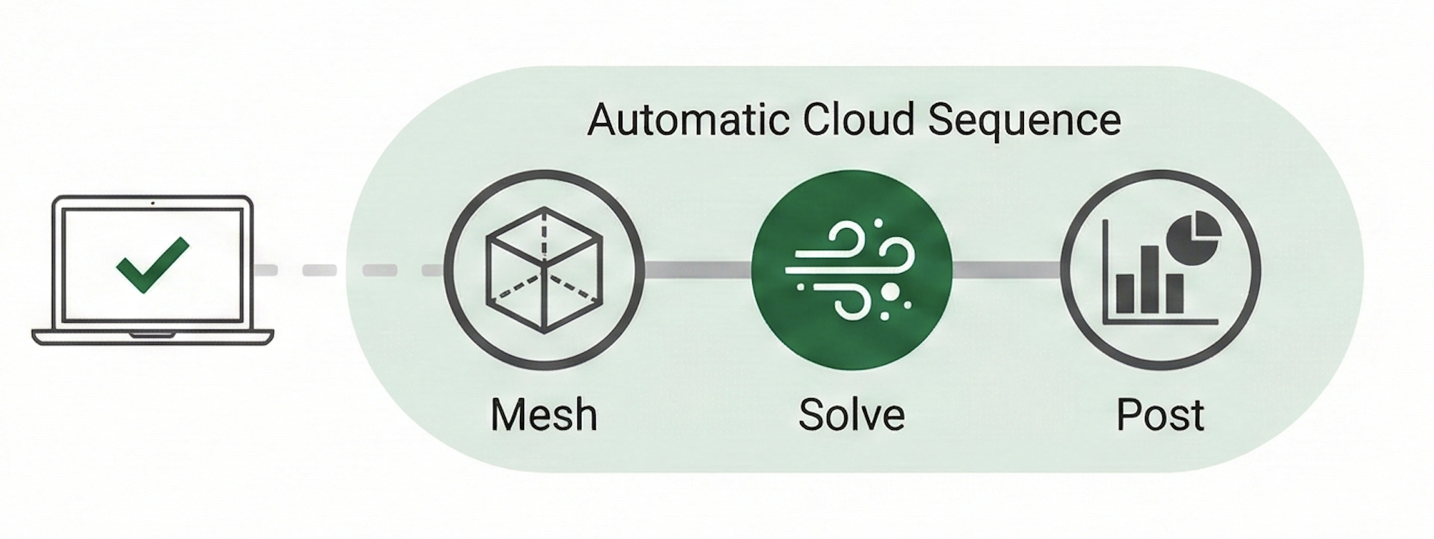
Once you submit a task—or a chain of tasks—you do not need to stay connected. You can define a full workflow (e.g., Import Geometry \(\rightarrow\) Generate Mesh \(\rightarrow\) Run Solver \(\rightarrow\) Extract Slices) and submit it all at once.
Offline Processing: You can close your browser or shut down your laptop immediately after submission.
Automatic Management: Our system orchestrates the steps. It waits for the mesh to finish before starting the solver, and waits for the solver to finish before generating reports.
Status Check: The system updates the progress in your project dashboard. You can log in at any time to check the status and retrieve results once the pipeline is complete.
The Solver Engine#
At the core of the platform is the proprietary Flow360 Solver.
Unstructured & Node-Based: The solver operates on unstructured grids, handling complex geometries without the limitations of structured block meshes.
Consistent & Repeatable: The solver is built to be hardware agnostic. While negligible differences may exist at the machine-precision level, the engineering results remain consistent down to very high precision. Re-running a simulation yields repeatable outcomes, ensuring that your design comparisons are valid regardless of the specific cloud hardware assigned to the task.
FlexCredits and Cost#
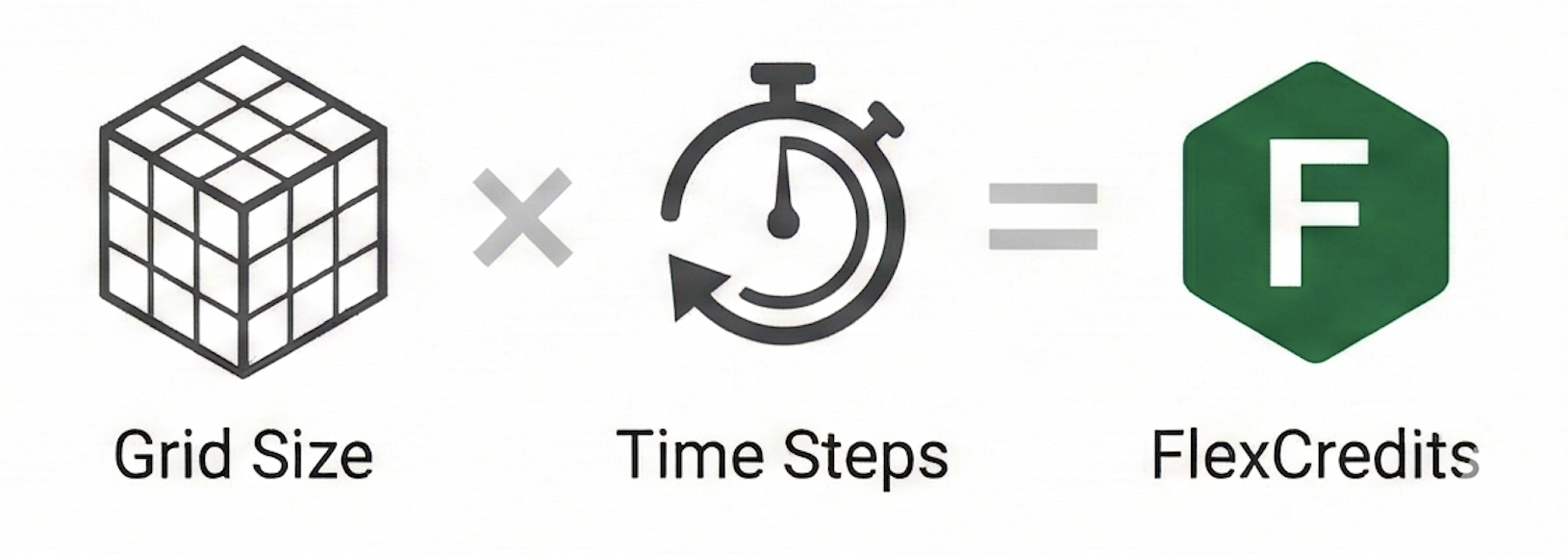
Flow360 uses a Physics-Based Pricing model called FlexCredits, rather than a hardware-rental model.
We do not charge based on “which GPU you used” or “how long the wall-clock ran.” Instead, the cost is proportional to the complexity of your physics:
(1)#\[\text{Cost} \propto (\text{Grid Size}) \times (\text{Number of Time Steps})\]
where:
Grid Size: The number of grid points (nodes) in your mesh.
Time Steps: The number of physical iterations (or pseudo-time steps for steady cases).
This means your costs are predictable based on your simulation setup, regardless of how fast the hardware executes the problem.
The charge for storage is the following:
resource |
storage price |
|---|---|
surface mesh |
free |
volume mesh |
free |
case |
0.00166 FlexUnit/GB/day (or 0.05 FlexUnit/GB/month) |
To reduce data storage costs we encourage users to:
Delete case if results will no longer be needed
Download results to local drive and delete case from Flow360