Conjugate Heat Transfer#
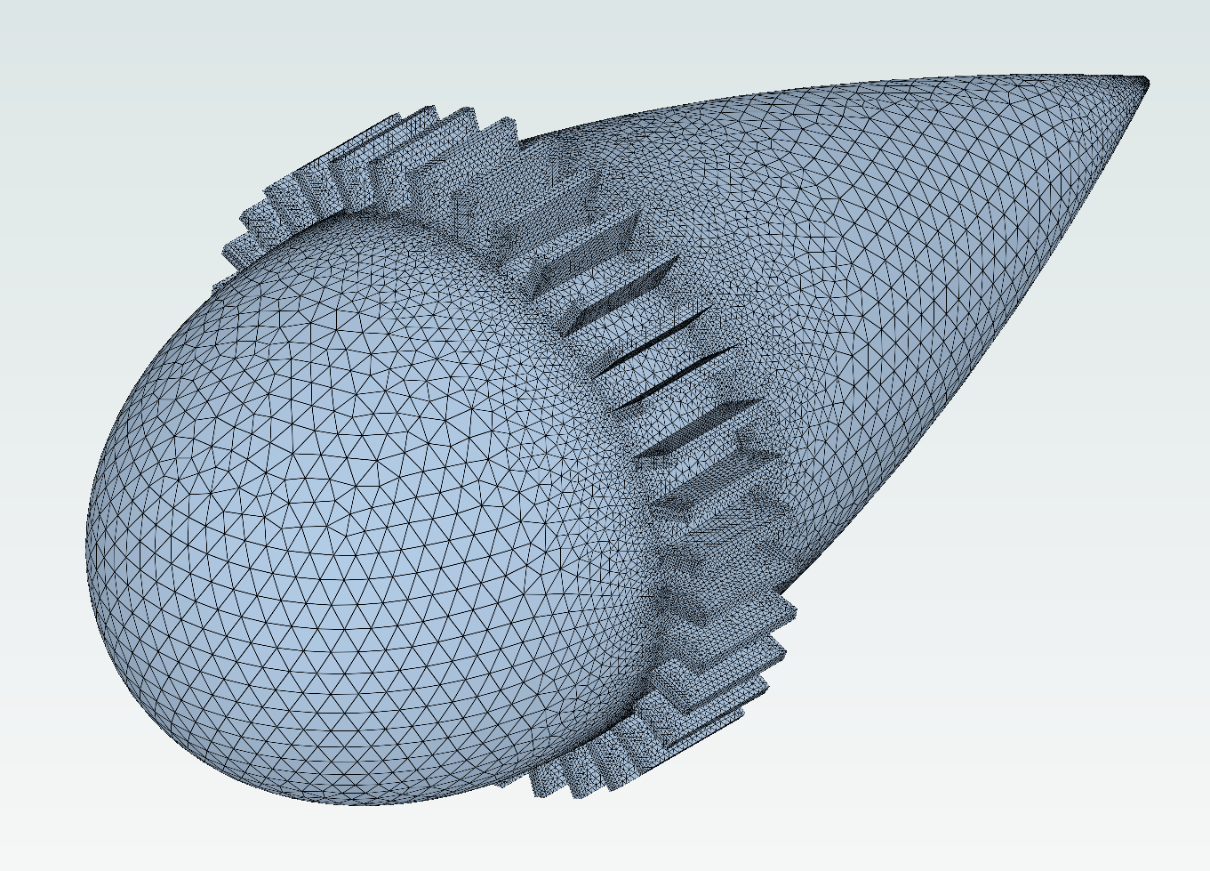
In this example we go over how to set up and perform a Conjugate Heat Transfer (CHT) simulation using Flow360 Python API. CHT is used to predict thermal interaction between a solid body and a fluid domain. We will go through creating a project, defining simulation settings, as well as post-processing results using the report functionality.

Note: The settings in this example are by no means a validation setup; they are crafted to showcase the capabilities of Flow360 and we have intentionally reduced node count and example FC cost. For rigorous validation, modify the settings as needed.
1. Setup and Imports#
First, we import the required modules from flow360 library.
[1]:
import flow360 as fl
from flow360 import u
from flow360.examples import TutorialCHTSolver
from flow360.plugins.report.report import ReportTemplate
from flow360.plugins.report.report_items import (
    Camera,
    Chart3D,
    FrontCamera,
    Inputs,
    LeftCamera,
    Settings,
    Summary,
)
2. Project Initialization#
A Project in Flow360 acts as a container for simulations and their related data. In this instance, the project is initialized directly from a pre-existing volume mesh file.
[2]:
TutorialCHTSolver.get_files()

project = fl.Project.from_volume_mesh(
    TutorialCHTSolver.mesh_filename, name="CHT results from Python"
)

volume_mesh = project.volume_mesh
[11:11:19] INFO: VolumeMesh successfully submitted:
                   type   = Volume Mesh
                   name   = CHT results from Python
                   id     = vm-8d68a03b-3db8-4913-abe5-e457188fa9ea
                   status = uploaded
3. Simulation Parameters Definition#
All parameters for the simulation exist within the SimulationParams object. In order to better focus on Solid model definition, we will define it a bit further down below.
Before that, we need to specify our Fluid domain solver settings and boundary conditions, operating condition of our simulation, as well as post-processing information such as reference geometry dimensions and outputs we want to get from the solver.
[3]:
with fl.SI_unit_system:
    params = fl.SimulationParams(
        reference_geometry=fl.ReferenceGeometry(
            moment_center=[0, 0, 0] * fl.u.m,
            moment_length=[1, 1, 1] * fl.u.m,
            area=1 * fl.u.m**2,
        ),
        operating_condition=fl.AerospaceCondition.from_mach(mach=0.1),
        time_stepping=fl.Steady(
            max_steps=10000, CFL=fl.RampCFL(initial=1, final=100, ramp_steps=1000)
        ),
        models=[
            fl.Fluid(
                navier_stokes_solver=fl.NavierStokesSolver(
                    absolute_tolerance=1e-9,
                    linear_solver=fl.LinearSolver(max_iterations=35),
                    order_of_accuracy=2,
                    kappa_MUSCL=-1,
                ),
                turbulence_model_solver=fl.SpalartAllmaras(
                    absolute_tolerance=1e-8,
                    linear_solver=fl.LinearSolver(max_iterations=25),
                    equation_evaluation_frequency=4,
                    order_of_accuracy=2,
                ),
            ),
            fl.Wall(
                surfaces=volume_mesh["fluid/centerbody"],
            ),
            fl.Freestream(
                surfaces=volume_mesh["fluid/farfield"],
            ),
        ],
        outputs=[
            fl.VolumeOutput(
                output_format="both",
                output_fields=[
                    "primitiveVars",
                    "T",
                    "Cp",
                    "Mach",
                ],
            ),
            fl.SurfaceOutput(
                surfaces=volume_mesh["*"],
                output_format="both",
                output_fields=["primitiveVars", "T", "Cp", "Cf", "CfVec"],
            ),
            fl.SliceOutput(
                entities=[
                    fl.Slice(
                        name="slice_x",
                        normal=(1, 0, 0),
                        origin=(0.35, 0, 0),
                    ),
                    fl.Slice(
                        name="slice_y",
                        normal=(0, 1, 0),
                        origin=(0, 0, 0),
                    ),
                ],
                output_fields=["T", "Mach"],
            ),
        ],
    )
[11:11:50] INFO: using: SI unit system for unit inference.
Solid Model#
The Solid model is used in CHT analysis. Its parameters define the thermal behavior of the solid body:
entities: Specifies which mesh regions are to be treated as solid. Here, the “solid” entity from the volume mesh is selected.heat_equation_solver: Configures the numerical solver for the heat equation within the solid. Parameters such as tolerance and linear solver iterations can be adjusted to control convergence.material: Defines the thermal properties of the solid material.SolidMaterialclass requires a name andthermal_conductivity.volumetric_heat_source: Allows for the specification of an internal heat generation rate within the solid’s volume, specified in Watts per cubic meter.
For solid surfaces not coupled with the fluid, an adiabatic condition is applied using a Wall boundary with a specified zero HeatFlux.
[4]:
with fl.SI_unit_system:
    models = [
        fl.Solid(
            entities=volume_mesh["solid"],
            heat_equation_solver=fl.HeatEquationSolver(
                absolute_tolerance=1e-11,
                linear_solver=fl.LinearSolver(
                    max_iterations=25,
                    absolute_tolerance=1e-12,
                ),
                equation_evaluation_frequency=10,
            ),
            material=fl.SolidMaterial(
                name="copper",
                thermal_conductivity=398 * fl.u.W / (fl.u.m * fl.u.K),
            ),
            volumetric_heat_source=5e3 * fl.u.W / (0.01257 * fl.u.m**3),
        ),
        fl.Wall(
            surfaces=volume_mesh["solid/adiabatic"],
            heat_spec=fl.HeatFlux(0 * fl.u.W / fl.u.m**2),
        ),
    ]

params.models.extend(models)
INFO: using: SI unit system for unit inference.
4. Case Execution#
We run the simulation by using project.run_case(). The script then calls case.wait() to wait until the simulation is finished on the Flow360 platform.
[5]:
case = project.run_case(params=params, name="CHT case from Python")

case.wait()
INFO: using: SI unit system for unit inference.
[11:11:52] INFO: Successfully submitted:
                   type   = Case
                   name   = CHT case from Python
                   id     = case-a12053be-2867-4159-8e28-1ba088a05062
                   status = pending
5. Results Post-Processing#
Upon completion, results can be accessed via the case.results attribute. Various data, such as surface heat transfer, can be retrieved.
[6]:
results = case.results

surface_heat_transfer = results.surface_heat_transfer.as_dataframe()
print(surface_heat_transfer)
[11:20:04] INFO: Saved to
           /var/folders/qk/mywsrvps5gl_f3yjx2k1v1xm0000gn/T/tmprcsk4uyf/c2da6cbc-1e41-4e8e-bdea-ce5549440fcc.csv
      physical_step  pseudo_step  fluid/Interface_solid_HeatTransferRate  \
0                 0            0                               -0.000111
1                 0           10                               -0.000144
2                 0           20                               -0.000109
3                 0           30                               -0.000118
4                 0           40                               -0.000105
...             ...          ...                                     ...
996               0         9960                               -0.000074
997               0         9970                               -0.000074
998               0         9980                               -0.000074
999               0         9990                               -0.000074
1000              0         9999                               -0.000074

      fluid/centerbody_HeatTransferRate  totalHeatFlux
0                             -0.000296            0.0
1                             -0.000140            0.0
2                             -0.000096            0.0
3                             -0.000068            0.0
4                             -0.000051            0.0
...                                 ...            ...
996                           -0.000001            0.0
997                           -0.000001            0.0
998                           -0.000001            0.0
999                           -0.000001            0.0
1000                          -0.000001            0.0

[1001 rows x 5 columns]
Report Preparation#
Flow360 includes a feature for automated report generation to visualize simulation outcomes. This involves defining cameras for different views and specifying chart objects that determine the content of the report.
[7]:
cases = [case]

exclude = ["fluid/farfield", "solid/interface_fluid", "solid/adiabatic"]

front_camera_slice = FrontCamera(dimension=1, dimension_dir="width")
side_camera_slice = LeftCamera(
    pan_target=(0.35, 0, 0), dimension=2, dimension_dir="width"
)
front_right_top_camera = Camera(
    position=(-1, -1, 1), look_at=(0.35, 0, 0), dimension=1, dimension_dir="width"
)
Report Item Configuration#
Chart3D objects are used to create three-dimensional visualizations of the results. Each chart can be configured to display specific data fields (e.g., temperature T) on selected surfaces or slices, with defined contour limits and camera views.
[8]:
x_slice_screenshot = Chart3D(
    section_title="Slice temperature at x=0.35",
    items_in_row=2,
    force_new_page=True,
    show="slices",
    include=["slice_x"],
    field="T",
    limits=(285 * u.K, 395 * u.K),
    camera=front_camera_slice,
    fig_name="slice_x",
)

y_slice_screenshot = Chart3D(
    section_title="Slice temperature at y=0",
    items_in_row=2,
    force_new_page=True,
    show="slices",
    include=["slice_y"],
    field="T",
    limits=(285 * u.K, 395 * u.K),
    camera=side_camera_slice,
    fig_name="slice_y",
)

surface_screenshot = Chart3D(
    section_title="Surface temperature",
    items_in_row=2,
    force_new_page=True,
    show="boundaries",
    field="T",
    limits=(285 * u.K, 395 * u.K),
    exclude=exclude,
    camera=front_right_top_camera,
)
Report Creation and Download#
ReportTemplate class is where we assemble all the defined charts and summary items into a complete report structure. Then, create_in_cloud method initiates the generation process. Once everything is done, a report PDF file will be automatically downloaded
[9]:
report = ReportTemplate(
    title="CHT results screenshots",
    items=[
        Summary(),
        Inputs(),
        x_slice_screenshot,
        y_slice_screenshot,
        surface_screenshot,
    ],
    settings=Settings(dpi=150),
)
report = report.create_in_cloud(
    "CHT, dpi=default",
    cases,
)

report.wait()
report.download("report.pdf")
[11:21:33] INFO: Saved to report.pdf
[9]:
'report.pdf'