Periodic BCs#
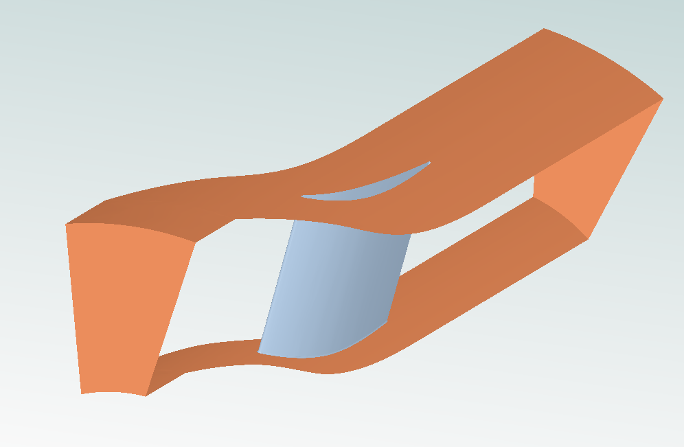
This notebook sets up a rotationally periodic steady-state simulation of the TU Berlin TurboLab Stator using the Flow360 Python API. It focuses on applying Periodic Boundary Conditions using rotational periodicity solver settings.
Note: The settings in this example are by no means a validation setup; they are crafted to showcase the capabilities of Flow360 and we have intentionally reduced node count and example FC cost. For rigorous validation, modify the settings as needed.
1. Imports and Project Setup#
We import the necessary Flow360 libraries and load the project geometry from the pre-existing volume mesh file provided by the TutorialPeriodicBC example module. The project is created directly from a pre generated volume mesh. The grid unit length is in millimeters (mm).
[1]:
import flow360 as fl
from flow360.examples import TutorialPeriodicBC

# Fetch the necessary volume mesh file
TutorialPeriodicBC.get_files()

# Create the project from the pre-existing volume mesh
project = fl.Project.from_volume_mesh(
    TutorialPeriodicBC.mesh_filename,
    length_unit="mm",
    name="Tutorial Periodic Boundary Condition from Python",
)

# Get the volume mesh object to define surfaces for models
volume_mesh = project.volume_mesh
[12:27:44] INFO: VolumeMesh successfully submitted:
                   type        = Volume Mesh
                   name        = Tutorial Periodic Boundary Condition from Python
                   id          = vm-e82bc122-d82d-449a-9bab-23b3ec2fcff4
                   status      = uploaded
                   project id  = prj-6d073a5d-7cca-4517-b25d-59ca8ae66623
2. Define the operating_condition simulation parameter#
We define the operating condition based on Mach number and Reynolds number. All definitions are in the standard SI unit system with the Reynolds reference length being the grid unit (mm).
[2]:
with fl.SI_unit_system:

    # Calculate full thermodynamic state from Mach and Reynolds numbers
    operating_condition = fl.AerospaceCondition.from_mach_reynolds(
        mach=0.13989,
        reynolds_mesh_unit=3200,
        project_length_unit=1 * fl.u.mm,
        temperature=298.25 * fl.u.K,
    )
[12:28:03] INFO: using: SI unit system for unit inference.
           INFO: Density and viscosity were calculated based on input data, ThermalState will be automatically
           created.
3. Define solver settings through the Fluid model#
We define detailed settings for the steady-state Navier-Stokes and Spalart-Allmaras turbulence solvers, including absolute tolerances, linear solver limits, and 2nd order accuracy.
[3]:
with fl.SI_unit_system:
    # Configure the Navier-Stokes solver for steady flow
    navier_stokes_solver = fl.NavierStokesSolver(
        absolute_tolerance=1e-11,
        linear_solver=fl.LinearSolver(max_iterations=20),
        order_of_accuracy=2,
        kappa_MUSCL=0.33,
        update_jacobian_frequency=1,
        equation_evaluation_frequency=1,
        numerical_dissipation_factor=1,
    )

    # Configure the Spalart-Allmaras turbulence model solver
    turbulence_model_solver = fl.SpalartAllmaras(
        absolute_tolerance=1e-10,
        linear_solver=fl.LinearSolver(max_iterations=20),
        update_jacobian_frequency=1,
        equation_evaluation_frequency=1,
        order_of_accuracy=2,
    )

    # Combine into a Fluid model
    fluid_model = fl.Fluid(
        navier_stokes_solver=navier_stokes_solver,
        turbulence_model_solver=turbulence_model_solver,
    )
INFO: using: SI unit system for unit inference.
4. Define Boundary Condition Models#
We assign boundary conditions to the surfaces defined in the volume mesh, including a crucial Periodic condition with rotational specification for the passage walls.
[4]:
with fl.SI_unit_system:
    models_list = [
        fluid_model,
        # Wall surfaces (vane, blade fillet, shroud, hub)
        fl.Wall(
            surfaces=[
                volume_mesh["fluid/vane_*"],
                volume_mesh["fluid/bladeFillet_*"],
                volume_mesh["fluid/shroud"],
                volume_mesh["fluid/hub"],
            ]
        ),
        # Freestream inlet condition
        fl.Freestream(
            surfaces=[
                volume_mesh["fluid/inlet"],
            ]
        ),
        # Outflow condition with specified static pressure
        fl.Outflow(
            surfaces=[
                volume_mesh["fluid/outlet"],
            ],
            spec=fl.Pressure(
                1.0032 * operating_condition.thermal_state.pressure
            ),  # Slightly above ambient
        ),
        # Slip walls for computational domain boundaries (top/bottom)
        fl.SlipWall(
            surfaces=[
                volume_mesh["fluid/bottomFront"],
                volume_mesh["fluid/topFront"],
            ]
        ),
    ]
INFO: using: SI unit system for unit inference.
Define the Periodic Boundary Condition#
The periodic boundary condition connects two sets of surfaces in the mesh that are opposite each other. We need to specify the two sets of faces and that the periodicity is rotational around the X-axis.
For more information on the periodic boundary conditions, refer to the Surface Models documentation.
[5]:
# Here we define the Periodic BC to connect the two periodic surfaces in the mesh.
models_list.append(
    # Rotational Periodic Boundary Condition
    fl.Periodic(
        surface_pairs=[
            (volume_mesh["fluid/periodic-1"], volume_mesh["fluid/periodic-2"])
        ],  # Connects the two radially oppose mesh surfaces
        spec=fl.Rotational(
            axis_of_rotation=(1, 0, 0)
        ),  # Specify rotation around X-axis
    ),
)
5. Define slice locations and outputs#
We specify the desired slice locations and the output fields for volume data (tecplot format), surface data, and slice data. This ensures we capture all relevant flow physics for post-processing.
[6]:
with fl.SI_unit_system:
    # Define slice planes for visualization and data extraction
    slice_inlet = fl.Slice(
        name="Inlet",
        normal=[1, 0, 0],
        origin=[-179, 0, 0] * fl.u.m,
    )
    slice_outlet = fl.Slice(
        name="Outlet",
        normal=[1, 0, 0],
        origin=[539, 0, 0] * fl.u.m,
    )
    slice_trailing_edge = fl.Slice(
        name="TrailingEdge",
        normal=[1, 0, 0],
        origin=[183, 0, 0] * fl.u.m,
    )
    slice_wake = fl.Slice(
        name="Wake",
        normal=[1, 0, 0],
        origin=[294.65, 0, 0] * fl.u.m,
    )
    outputs_list = [
        # Full Volume Output for 3D visualization (Tecplot recommended)
        fl.VolumeOutput(
            output_format=["tecplot"],
            output_fields=[
                "primitiveVars",
                "vorticity",
                "Cp",
                "Mach",
                "qcriterion",
                "mut",
                "nuHat",
                "mutRatio",
                "gradW",
                "T",
                "residualNavierStokes",
            ],
        ),
        # Surface Output for wall quantities
        fl.SurfaceOutput(
            surfaces=volume_mesh["*"],
            output_format=["paraview", "tecplot"],
            output_fields=[
                "primitiveVars",
                "Cp",
                "Cf",
                "CfVec",
                "yPlus",
                "nodeForcesPerUnitArea",
            ],
        ),
        # Slice Output for 2D flow field investigation
        fl.SliceOutput(
            slices=[slice_inlet, slice_outlet, slice_trailing_edge, slice_wake],
            output_format=["paraview", "tecplot"],
            output_fields=["Cp", "primitiveVars", "T", "Mach", "gradW"],
        ),
    ]
INFO: using: SI unit system for unit inference.
6. Construct Final Simulation Parameters#
We combine all the previously defined components—geometry, operating condition, time stepping (Steady), models, and outputs—into the final SimulationParams object.
[7]:
with fl.SI_unit_system:
    params = fl.SimulationParams(
        reference_geometry=fl.ReferenceGeometry(
            moment_center=[0, 0, 0], moment_length=[1, 1, 1], area=209701.3096271187
        ),
        operating_condition=operating_condition,
        time_stepping=fl.Steady(max_steps=5000, CFL=fl.AdaptiveCFL()),
        models=models_list,
        outputs=outputs_list,
    )
INFO: using: SI unit system for unit inference.
7. Run the Case 🏃#
Finally, we submit the simulation using the configured parameters to Flow360.
[8]:
case = project.run_case(
    params=params, name="Tutorial Periodic Boundary Condition from Python"
)
           INFO: Density and viscosity were calculated based on input data, ThermalState will be automatically
           created.
INFO: using: SI unit system for unit inference.
[12:28:05] INFO: Successfully submitted:
                   type        = Case
                   name        = Tutorial Periodic Boundary Condition from Python
                   id          = case-994ad1dc-1fc0-4e42-9d25-2e609778f2e8
                   status      = pending
                   project id  = prj-6d073a5d-7cca-4517-b25d-59ca8ae66623
While we wait for the case to finish, we invite you to monitor the case in the Flow360 GUI. Once finished, you can easily post-process the results after completion.
[9]:
# wait until the case finishes execution
case.wait()
results = case.results
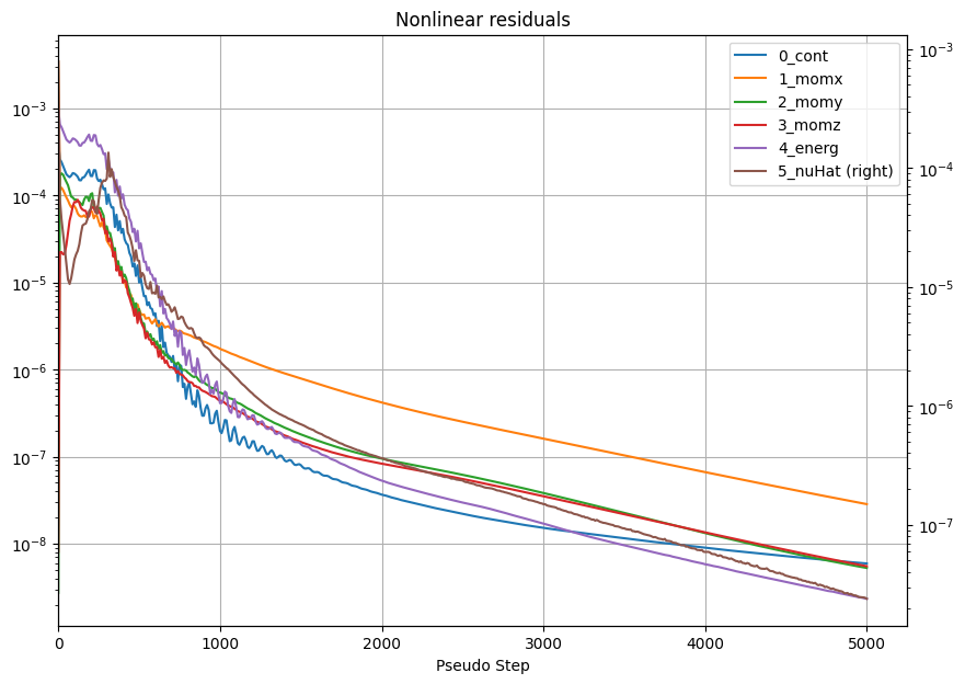
# nonlinear residuals contain convergence information
nonlinear_residuals = results.nonlinear_residuals.as_dataframe()
ax = nonlinear_residuals.plot(
x="pseudo_step",
y=["0_cont", "1_momx", "2_momy", "3_momz", "4_energ", "5_nuHat"],
xlim=(0, None),
xlabel="Pseudo Step",
secondary_y=["5_nuHat"],
figsize=(10, 7),
logy=True,
title="Nonlinear residuals",
)
ax.grid(True)
[12:33:31] INFO: Saved to /tmp/tmpk0dinw1f/d01c7941-039c-4eda-bd68-fef55912ced2.csv
[ ]: