Dynamic Derivatives Using Sliding Interfaces#
This notebook demonstrates how to obtain dynamic stability derivatives by simulating unsteady flow over a NACA0012 wing that pitches back and forth within a sliding interface.
Geometry#
The wing geometry has:
Chord \(c\) = 1 m
Span \(b\) = 2 m
Reference area \(A_{ref}\) = 2 m²
Moment length = [\(b\)/2, \(c\), \(b\)/2] = [1, 1, 1] m
Moment center = [0, 0, 0] (at quarter-chord, midspan)
Simulation Strategy#
Steady Initialization:
Ramp CFL from 1 to 100 over 1000 steps for robust convergence
Fixed sliding interface (zero angular velocity) to establish baseline flow
Maximum 10000 steps to ensure convergence
Unsteady Oscillation:
Sliding interface updated to oscillating motion
Sinusoidal pitching with amplitude 2° and frequency 2.5 flowthru/rad
400 time steps (4 complete cycles)
Note: The settings in this example are by no means a validation setup; they are crafted to showcase the capabilities of Flow360 and we have intentionally reduced node count and example FC cost. For rigorous validation, modify the settings as needed.
1. Download tutorial files#
[1]:
import math
import flow360 as fl
from flow360.examples import TutorialDynamicDerivatives

TutorialDynamicDerivatives.get_files()
The downloaded files include the geometry (CSM format) for the NACA0012 wing.
2. Create project from geometry#
[2]:
project = fl.Project.from_geometry(
    TutorialDynamicDerivatives.geometry,
    name="Tutorial Calculating Dynamic Derivatives using Sliding Interfaces from Python",
)
geometry = project.geometry
geometry.group_faces_by_tag("faceName")
[09:57:06] INFO: Geometry successfully submitted:
                   type        = Geometry
                   name        = Tutorial Calculating Dynamic Derivatives using Sliding Interfaces from Python
                   id          = geo-e863d8e0-f3b6-4dd9-ba79-ff8cb38d3272
                   status      = uploaded
                   project id  = prj-9f2dbc33-dc46-4fa8-a385-82b4f61cc317
INFO: Waiting for geometry to be processed.
The wing is enclosed in a cylindrical sliding interface as shown below:
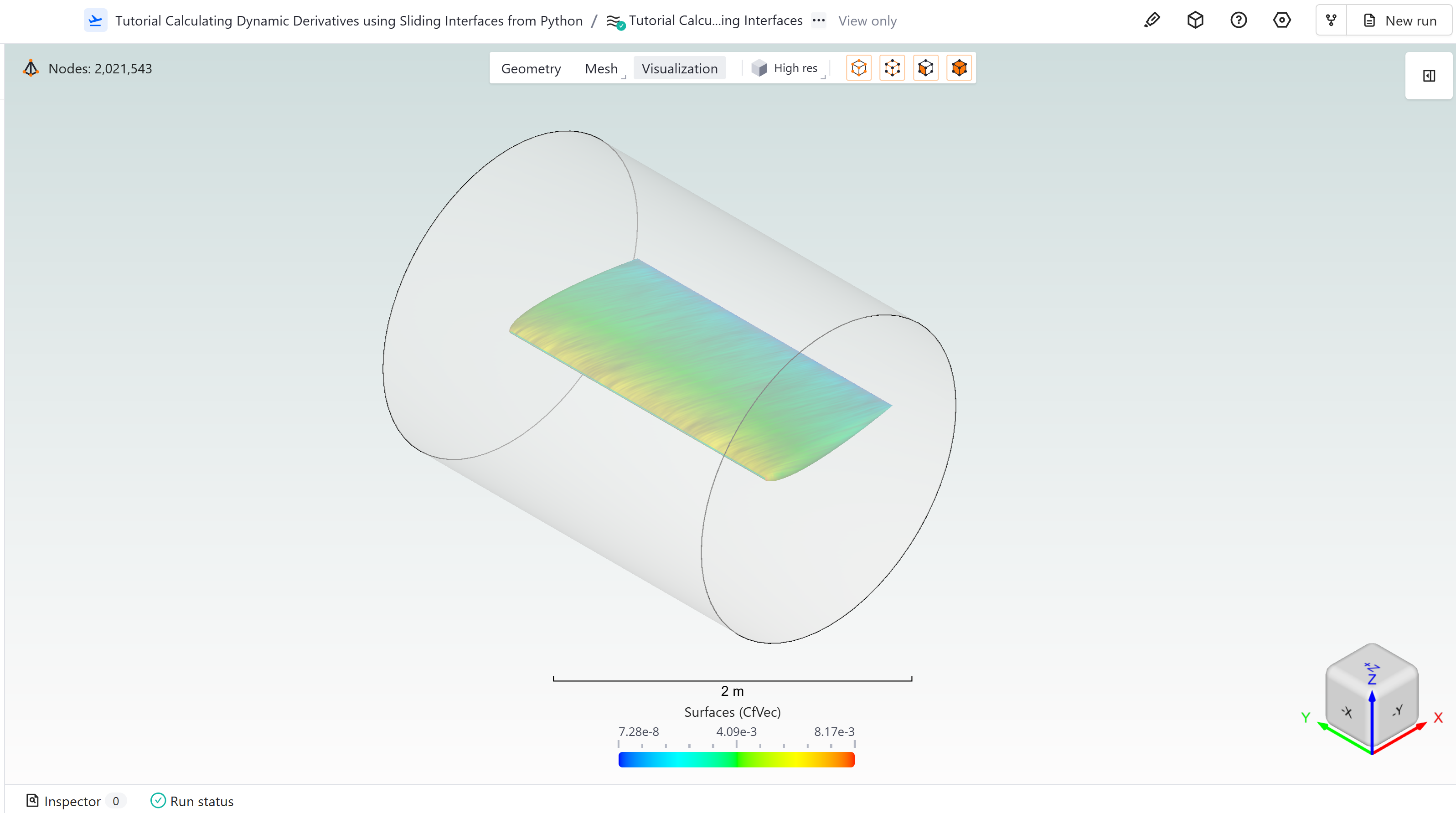
Figure: Wing enclosed in cylindrical sliding interface. The interface rotates about the y-axis, causing the wing to pitch.
3. Define sliding interface and meshing parameters#
The wing is enclosed in a cylindrical sliding interface:
Radius = 1.0 m
Height = 2.5 m
Rotation center = [0, 0, 0]
Rotation axis = y-axis [0, 1, 0]
[3]:
with fl.SI_unit_system:
    cylinder = fl.Cylinder(
        name="cylinder",
        axis=[0, 1, 0],
        center=[0, 0, 0],
        inner_radius=0,
        outer_radius=1.0,
        height=2.5,
    )
    sliding_interface = fl.RotationVolume(
        spacing_axial=0.04,
        spacing_radial=0.04,
        spacing_circumferential=0.04,
        entities=cylinder,
        enclosed_entities=geometry["wing"],
    )
    farfield = fl.AutomatedFarfield(name="farfield")
[09:57:33] INFO: using: SI unit system for unit inference.
Key meshing parameters:
Automated meshing with sliding interface and farfield zones
Refined leading and trailing edges for accuracy
Boundary layer resolved with first layer thickness of 1e-6 m
[4]:
with fl.SI_unit_system:
    meshing_params = fl.MeshingParams(
        defaults=fl.MeshingDefaults(
            surface_max_edge_length=0.03 * fl.u.m,
            curvature_resolution_angle=8 * fl.u.deg,
            surface_edge_growth_rate=1.15,
            boundary_layer_first_layer_thickness=1e-6,
            boundary_layer_growth_rate=1.15,
        ),
        refinement_factor=1.0,
        volume_zones=[sliding_interface, farfield],
        refinements=[
            fl.SurfaceEdgeRefinement(
                name="leadingEdge",
                method=fl.AngleBasedRefinement(value=1 * fl.u.degree),
                edges=geometry["leadingEdge"],
            ),
            fl.SurfaceEdgeRefinement(
                name="trailingEdge",
                method=fl.HeightBasedRefinement(value=0.001),
                edges=geometry["trailingEdge"],
            ),
        ],
    )
INFO: using: SI unit system for unit inference.
4. Run steady case to initialize the flow field#
First, we run a steady case with a fixed sliding interface (zero angular velocity) to initialize the flow field. This provides a converged solution to start the unsteady simulation.
[5]:
with fl.SI_unit_system:
    params = fl.SimulationParams(
        meshing=meshing_params,
        reference_geometry=fl.ReferenceGeometry(
            moment_center=[0, 0, 0],
            moment_length=[1, 1, 1],
            area=2,
        ),
        operating_condition=fl.AerospaceCondition(
            velocity_magnitude=50,
        ),
        time_stepping=fl.Steady(
            max_steps=10000,
            CFL=fl.RampCFL(initial=1, final=100, ramp_steps=1000),
        ),
        outputs=[
            fl.VolumeOutput(name="VolumeOutput", output_fields=["Mach"]),
            fl.SurfaceOutput(
                name="SurfaceOutput",
                surfaces=geometry["*"],
                output_fields=["Cp", "CfVec"],
            ),
        ],
        models=[
            fl.Rotation(
                volumes=cylinder,
                spec=fl.AngularVelocity(0 * fl.u.rad / fl.u.s),
            ),
            fl.Freestream(surfaces=farfield.farfield, name="Freestream"),
            fl.Wall(surfaces=geometry["wing"], name="NoSlipWall"),
            fl.Fluid(
                navier_stokes_solver=fl.NavierStokesSolver(
                    absolute_tolerance=1e-9,
                    linear_solver=fl.LinearSolver(max_iterations=35),
                ),
                turbulence_model_solver=fl.SpalartAllmaras(
                    absolute_tolerance=1e-8,
                    linear_solver=fl.LinearSolver(max_iterations=25),
                ),
            ),
        ],
    )

project.run_case(
    params=params, name="Tutorial Dynamic Derivatives - Steady Initialization"
)

steady_case = fl.Case.from_cloud(project.case.id)
INFO: using: SI unit system for unit inference.
INFO: using: SI unit system for unit inference.
[09:57:36] INFO: Successfully submitted:
                   type        = Case
                   name        = Tutorial Dynamic Derivatives - Steady Initialization
                   id          = case-fc35883b-74e5-4ac9-9697-17e0a3e6a1bc
                   status      = pending
                   project id  = prj-9f2dbc33-dc46-4fa8-a385-82b4f61cc317
5. Understanding the Oscillation Setup#
The sliding interface oscillates according to the angle expression:
Where:
\(A\) = 0.0349066 rad (equivalent to 2°) - amplitude of oscillation
\(\omega_\text{non-dim}\) = nondimensional angular frequency
\(t_\text{non-dim}\) = nondimensional time
Calculating the nondimensional frequency:
We want the wing to complete one oscillation cycle over a specific number of flowthroughs. In this example, we use \(n\) = 2.5 flowthru/rad, meaning when \(\omega \cdot t\) changes by 1 radian, the air flows through 2.5 chord lengths.
Given:
Freestream velocity \(U_\infty\) = 50 m/s
Chord \(c\) = 1 m
Speed of sound \(C_\infty\) = 340.294 m/s
Grid unit \(L_\text{gridUnit}\) = 1 m
Physical angular frequency:
Nondimensional angular frequency:
Time step size:
We split each oscillation period into 100 steps:
6. Run unsteady case with oscillating interface#
Now we update the simulation parameters for the unsteady case and fork from the steady solution. Only the time stepping and rotation spec need to be modified.
[6]:
# Update parameters for unsteady case
with fl.SI_unit_system:
    params.time_stepping = fl.Unsteady(
        max_pseudo_steps=80,
        steps=400,
        step_size=0.01 * 2.0 * math.pi / 20.0 * fl.u.s,
        CFL=fl.RampCFL(initial=1, final=1e8, ramp_steps=20),
    )
    params.models[0].spec = fl.AngleExpression("0.0349066 * sin(0.05877271 * t)")

# Run unsteady case forked from steady solution
project.run_case(
    params=params,
    name="Tutorial Dynamic Derivatives - Unsteady Oscillation",
    fork_from=steady_case,
)
unsteady_case = project.case
INFO: using: SI unit system for unit inference.
INFO: using: SI unit system for unit inference.
[09:57:37] INFO: using: SI unit system for unit inference.
[09:57:38] INFO: Successfully submitted:
                   type        = Case
                   name        = Tutorial Dynamic Derivatives - Unsteady Oscillation
                   id          = case-e040a828-b521-432a-8402-5e1c58dcb612
                   status      = pending
                   project id  = prj-9f2dbc33-dc46-4fa8-a385-82b4f61cc317
7. Postprocessing - Extract Dynamic Derivatives#
Once the simulation is complete, we download the results and calculate the dynamic derivatives. The key output is the total_forces data which contains force and moment coefficients at each time step.
[7]:
import flow360 as fl
import numpy as np
import pandas as pd
import matplotlib.pyplot as plt

cmap = plt.colormaps["tab10"]

# Load completed example case from the example library (flow360 25.8 or above)
project = fl.Project.from_example(by_name="Dynamic Derivatives")
case = project.get_case()

# Note that in this example we're loading a pre-computed unsteady case from the example library,
# so the reader doesn't need to wait for the simulation to finish.
# For production usage, the user can use:
# case = unsteady_case
# or:
# case = fl.Case.from_cloud("your-case-id")

# Download and load results
case.results.total_forces.download(to_file="total_forces.csv")
case.results.total_forces.load_from_local("total_forces.csv")
total_forces = case.results.total_forces.as_dataframe()
           INFO: Found closest match for 'Dynamic Derivatives': 'Calculating Dynamic Derivatives using Sliding
           Interfaces' (similarity: 50.67 %)
[09:57:39] INFO: Copy operation started for project prj-0ad2a0d2-873f-43cc-b38a-a4e4e7b7268c. Waiting for
           completion...
[09:57:51] INFO: Copy operation completed successfully.
[09:57:53] INFO: Saved to total_forces.csv
Extract unique physical steps#
The total_forces data contains multiple rows per physical step (one per pseudo-step). We extract the final converged value at each physical step.
[8]:
def extract_unique_physical_steps(input_df):
    """Extract the row at the last pseudo step at the end of each physical step."""
    physical_steps_raw = input_df["physical_step"]
    n_rows = len(physical_steps_raw)
    selected_row_index = []
    for i in range(n_rows - 1):
        if physical_steps_raw.iloc[i + 1] > physical_steps_raw.iloc[i]:
            selected_row_index.append(i)
    selected_row_index.append(n_rows - 1)
    output = pd.DataFrame()
    for k, v in input_df.items():
        output[k] = [v.iloc[j] for j in selected_row_index]
    return output.reset_index(drop=True)


total_forces = extract_unique_physical_steps(total_forces)
print(f"Number of physical steps: {len(total_forces)}")
Number of physical steps: 400
Calculate nondimensional time, angle of attack, and pitch rate#
We compute:
Nondimensional time from physical steps
Angle of attack \(\alpha = A \sin(\omega t)\)
Pitch rate \(\dot{\alpha}\) using central differences, converted to rad/flowthru
[9]:
# Define simulation parameters
length_unit = case.params.private_attribute_asset_cache.project_length_unit  # m
U_inf = case.params.operating_condition.velocity_magnitude  # m/s
C_inf = 340.29400580821283 * fl.u.m / fl.u.s  # speed of sound
n_chord_per_period = 2.5  # flowthru/rad
chord = 1 * fl.u.m

omega_physical = U_inf / (n_chord_per_period * chord)  # 1/s
omega_nondim = omega_physical / (C_inf / length_unit)
time_step_size_nondim = 0.01 * 2 * np.pi / omega_nondim  # nondim

amplitude_deg = 2 * fl.u.deg
amplitude_rad = amplitude_deg.to(fl.u.rad)


def compute_time_nondim(df):
    """Compute nondimensional time from physical step."""
    n_steps = len(df["physical_step"])
    df["time_nondim"] = np.zeros(n_steps)
    for i in range(n_steps):
        df.loc[i, "time_nondim"] = time_step_size_nondim * (
            df.loc[i, "physical_step"] + 1
        )


def compute_alpha_dot(df):
    """Compute angle of attack and pitch rate."""
    n_steps = len(df["physical_step"])
    df["alpha"] = np.zeros(n_steps)
    df["alpha_dot"] = np.zeros(n_steps)
    alpha_eq_0_index = []

    # Compute alpha
    for i in range(n_steps):
        t = df.loc[i, "time_nondim"]
        df.loc[i, "alpha"] = amplitude_rad * np.sin(omega_nondim * t)

    # Compute alpha_dot using central difference
    for i in range(1, n_steps - 1):
        df.loc[i, "alpha_dot"] = (
            (df.loc[i + 1, "alpha"] - df.loc[i - 1, "alpha"])
            / (2 * time_step_size_nondim)
            * C_inf
            / length_unit
            * chord
            / U_inf
        )
        if abs(df.loc[i, "alpha"]) < 1e-10:
            alpha_eq_0_index.append(i)

    return alpha_eq_0_index


compute_time_nondim(total_forces)
alpha_eq_0_index = compute_alpha_dot(total_forces)
print(f"Found {len(alpha_eq_0_index)} points where alpha = 0")
[09:57:54] INFO: using: SI unit system for unit inference.
Found 7 points where alpha = 0
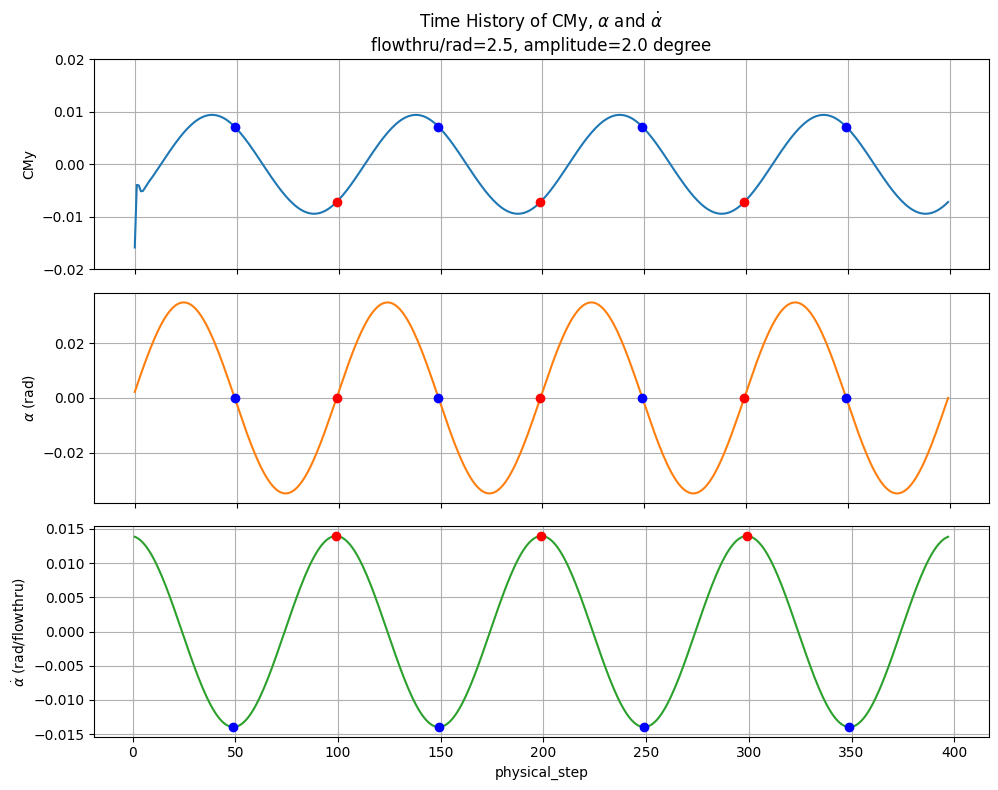
Plot time history#
Plot the time history of the pitch moment coefficient \(C_{My}\), angle of attack \(\alpha\), and pitch rate \(\dot{\alpha}\). The blue and red dots mark the points where \(\alpha = 0\) (extrema of \(\dot{\alpha}\)).
[10]:
def plot_time_history(df, alpha_eq_0_idx):
    _, axs = plt.subplots(3, figsize=(10, 8))

    # Time history of CMy
    axs[0].plot(df["physical_step"], df["CMy"], color=cmap.colors[0])
    axs[0].set_yticks(np.linspace(-0.02, 0.02, 5))
    axs[0].set_ylim([-0.02, 0.02])
    axs[0].set_ylabel("CMy")

    # Time history of alpha
    axs[1].plot(df["physical_step"], df["alpha"], color=cmap.colors[1])
    axs[1].set_ylabel(r"$\alpha$ (rad)")

    # Time history of alpha_dot
    axs[2].plot(df["physical_step"][1:-2], df["alpha_dot"][1:-2], color=cmap.colors[2])
    axs[2].set_ylabel(r"$\dot{\alpha}$ (rad/flowthru)")
    axs[2].set_xlabel("physical_step")

    for ax in axs:
        ax.label_outer()
        ax.grid()

    # Mark alpha=0 points (blue for min alpha_dot, red for max alpha_dot)
    for i in alpha_eq_0_idx:
        color = "b" if df["alpha_dot"][i] < 0 else "r"
        axs[0].plot(df["physical_step"][i], df["CMy"][i], "o", color=color)
        axs[1].plot(df["physical_step"][i], df["alpha"][i], "o", color=color)
        axs[2].plot(df["physical_step"][i], df["alpha_dot"][i], "o", color=color)

    axs[0].set_title(
        r"Time History of CMy, $\alpha$ and $\dot{\alpha}$"
        + "\n"
        + f"flowthru/rad={n_chord_per_period:.1f}, amplitude={amplitude_deg:.1f}"
    )
    plt.tight_layout()
    plt.show()


plot_time_history(total_forces, alpha_eq_0_index)
Extract dynamic derivative#
Plot \(C_{My}\) vs \(\dot{\alpha}\) for the last oscillation period and compute the dynamic derivative \(\frac{dC_{My}}{dq}\) from linear regression at \(\alpha = 0\).
[11]:
def plot_CMy_vs_q(df, alpha_eq_0_idx):
    plt.figure(figsize=(8, 6))

    # Plot CMy versus alpha_dot for the last period
    n_steps = len(df["physical_step"])
    begin = n_steps - 201
    end = n_steps - 1
    alpha_dot = df.loc[begin:end, "alpha_dot"]
    CMy = df.loc[begin:end, "CMy"]
    plt.plot(alpha_dot, CMy, ".")

    # Extract alpha=0 points in the last period
    x = []
    y = []
    for i in alpha_eq_0_idx:
        if i >= begin and i <= end:
            x.append(df.loc[i, "alpha_dot"])
            y.append(df.loc[i, "CMy"])

    # Mark the alpha=0 points
    plt.plot(x[0], y[0], "o", color="r", markersize=10)
    plt.plot(x[1], y[1], "o", color="b", markersize=10)

    # Linear regression through alpha=0 points
    coef = np.polyfit(x, y, 1)
    func = np.poly1d(coef)
    x_line = np.linspace(-0.02, 0.02, 101)
    plt.plot(x_line, func(x_line), "--", label=f"slope = {coef[0]:.3f}", color="k")

    # Formatting
    plt.xlabel(r"$\dot{\alpha} = q$ (deg/flowthru)")
    plt.ylabel("CMy")
    plt.ylim([-0.02, 0.02])
    plt.yticks(np.linspace(-0.02, 0.02, 5))
    plt.grid()
    plt.legend(loc="lower left")
    plt.title(
        f"Dynamic Derivative dCMy/dq\nflowthru/rad={n_chord_per_period:.1f}, amplitude={amplitude_deg:.1f}"
    )

    # Set x-axis to deg/flowthru
    tick_locations = np.linspace(-1, 1, 5) / 180 * np.pi
    ax = plt.gca()
    ax.set_xticks(
        tick_locations, [f"{loc * 180 / np.pi:.1f}" for loc in tick_locations]
    )

    # Add text annotations
    ax.text(
        -0.016,
        0.01,
        r"$\alpha = 0$" + "\n" + r"min $\dot{\alpha}$",
        fontsize=14,
        color="b",
    )
    ax.text(
        +0.012,
        -0.014,
        r"$\alpha = 0$" + "\n" + r"max $\dot{\alpha}$",
        fontsize=14,
        color="r",
    )

    plt.tight_layout()
    plt.show()

    print(f"\nDynamic derivative: dCMy/dq = {coef[0]:.3f}")


plot_CMy_vs_q(total_forces, alpha_eq_0_index)
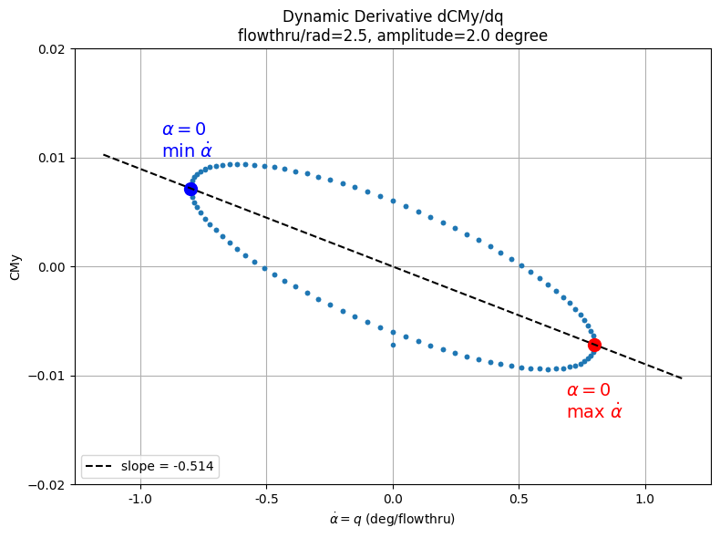
Dynamic derivative: dCMy/dq = -0.514
Summary#
This notebook demonstrated the complete workflow for calculating dynamic derivatives using Flow360:
Download Tutorial Files: Obtained the NACA0012 wing geometry (CSM format)
Create Project: Set up a Flow360 project from the geometry
Define Sliding Interface and Meshing: Configured the cylindrical sliding interface enclosing the wing, farfield zone, and mesh refinements
Run Steady Case: Initialized the flow field with a fixed sliding interface (zero angular velocity)
Understanding Oscillation Setup: Calculated nondimensional frequency and time step for sinusoidal pitching motion
Run Unsteady Case: Forked from steady solution and ran 400 time steps (4 complete cycles) with oscillating interface
Postprocessing: Extracted dynamic derivatives from force history
Extracted unique physical steps from force history
Computed angle of attack \(\alpha\) and pitch rate \(\dot{\alpha}\)
Extracted dynamic derivative from linear fit at \(\alpha = 0\)
Key Result: The dynamic pitching moment derivative is approximately:
This derivative is critical for:
Flight dynamics modeling
Stability and control analysis
Control system design
Aircraft certification