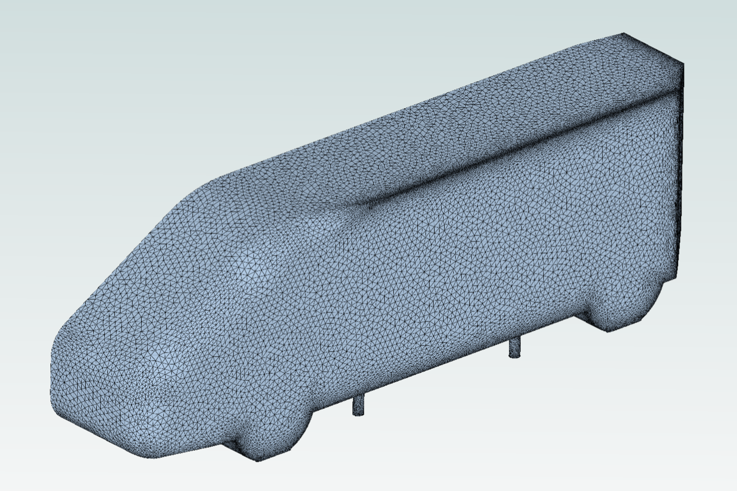
Windsor Body#
This notebook demonstrates three powerful features of the Flow360 software:
Geometry AI
Solution Interpolation
Custom Stopping Criteria
Geometry AI is a powerful tool in Flow360 that enables more robust and easier meshing of complex geometries. It automatically handles geometry processing challenges such as:
Complex geometric transformations (translation, rotation, mirroring)
Boolean operations between multiple bodies
Automatic gap sealing and geometry repair
Intelligent meshing parameter selection
Solution Interpolation allows users to transfer the solution between similar meshes to speed up convergence. When coupled with Custom Stopping Criteria, this can significantly reduce the cost and time of design iteration studies.
The example showcases a Windsor body with wheels, where we:
Load geometry from multiple files (main body and wheel)
Transform and mirror the wheel to create front and rear wheels
Merge the wheels with the main body using boolean operations
Set up and run a CFD simulation with custom stopping criteria based on a drag coefficient convergence
Apply a rotation transformation to change the toe angle of the wheels
Interpolate a solution from the straight-wheel case to the turned-wheel case
Note: The settings in this example are by no means a validation setup; they are crafted to showcase the capabilities of Flow360 and we have intentionally reduced node count and example FC cost. For rigorous validation, modify the settings as needed.
1. Project Setup#
The next code cell imports the Flow360 Python API and creates a project from geometry files.
We’ll work with two geometry files:
windsorBody.stp: The main vehicle bodywheel.stl: A single wheel that will be positioned and mirrored to create front and rear wheels
The project is initialized with the geometry files, specifying the length unit (millimeters) and a project name.
[1]:
import flow360 as fl
from flow360.examples import Windsor
Windsor.get_files()

# Create project from geometry files
prj = fl.Project.from_geometry(
    Windsor.geometry, # contains the chassis and the wheel files
    length_unit='mm',
    name="WindsorWithWheels",
)

geometry = prj.geometry
[11:32:17] INFO: The file (windsorBody.stp) is being downloaded, please wait.
[11:32:19] INFO: The file (wheel.stl) is being downloaded, please wait.
[11:32:45] INFO: Geometry successfully submitted:
                   type        = Geometry
                   name        = WindsorWithWheels
                   id          = geo-46949934-e7b6-4e17-be77-71530228e58c
                   status      = uploaded
                   project id  = prj-55981602-30d5-426e-9edf-ffc382a2a2be
INFO: Waiting for geometry to be processed.
2. Create Draft#
A draft is a working copy of the geometry that allows you to perform geometric transformations and modifications before meshing. The create_draft() function creates a draft from the geometry, enabling you to:
Transform geometry: Apply translations, rotations, and scaling to individual body groups
Mirror bodies: Create symmetric copies of geometry components
Configure boolean operations: Set which bodies to include in the final mesh via
mesh_exteriorflags
The draft workflow separates geometry manipulation from the original geometry files, allowing you to experiment with different configurations without modifying your source files. In this example, we’ll use the draft to position and mirror the wheel, then merge it with the main body.
[2]:
draft = fl.create_draft(
    new_run_from=geometry,
    face_grouping='groupByBodyId',
    edge_grouping='edgeId'
)
[11:33:05] INFO: Regrouping face entities under `groupByBodyId` tag (previous `faceId`).
           INFO: Creating draft with geometry grouping:
             faces: groupByBodyId
             edges: edgeId
             bodies: groupByFile
3. Geometry Processing#
This section demonstrates geometry manipulations in Flow360.
3.1 Coordinate Transformations#
The draft workflow allows geometric transformations without modifying the original geometry files:
Coordinate system assignment: Positions the wheel from the origin to its correct location relative to the vehicle body. This is accomplished using the
coordinate_systems.assign()method, which applies translations, rotations, and scaling to the selected entities. In this example, the front wheel is translated to its correct position using a custom coordinate system with a specific translation vector.
3.2 Mirroring#
Mirroring creates symmetric copies of geometry components about a specified plane:
Mirror plane definition: A
MirrorPlaneis defined with a normal vector and center point. The normal vector determines the orientation of the mirror plane, while the center point defines its position in 3D space.Symmetric geometry creation: The
mirror.create_mirror_of()function generates mirrored body groups from the original entities. This is particularly useful for symmetric geometries like vehicles, where components such as wheels can be duplicated on the opposite side with perfect symmetry. In this example, the rear wheel is created by mirroring the front wheel about a plane with normal(1, 0, 0), effectively creating a reflection along the x-axis.Automatic naming: Mirrored body groups are automatically assigned names based on the original entity name with a
_<mirror>suffix, making them easy to reference in subsequent operations like boundary condition assignment.
3.3 Boolean Operations#
Geometry AI excels at handling boolean operations between complex bodies:
Mesh exterior flags: By setting
windsor_body.mesh_exterior = Trueandfront_wheel.mesh_exterior = True, we want to mesh the volume which is the union of wheel and the Windsor body.Automatic intersection handling: Geometry AI automatically detects and resolves intersections between the wheels and body, creating clean surfaces for meshing. The complex intersections between the Windsor body and wheels are handled easily, ensuring smooth transitions and high-quality mesh generation at these critical interface regions. In fact, edges are not explicitly retained but they are ‘blended’ up to geometry accuracy.
Gap sealing: Small gaps at wheel-body interfaces are automatically sealed, preventing mesh generation failures
[3]:
# Process geometry using draft with Geometry AI
# Access body groups
with draft:
    windsor_body = draft.body_groups["windsorBody.stp"]
    front_wheel = draft.body_groups["wheel.stl"]

    # Translate front wheel to its position
    draft.coordinate_systems.assign(
        entities=front_wheel,
        coordinate_system=fl.CoordinateSystem(
            name="shift",
            reference_point=[0, 0, 0] * fl.u.mm,
            axis_of_rotation=(0, 0, 1),
            angle_of_rotation=0 * fl.u.deg,
            scale=(1.0, 1.0, 1.0),
            translation=[-320.025, -167, 70] * fl.u.mm
        )
    )

    # Create rear wheel by mirroring the front wheel
    mirror_plane = fl.MirrorPlane(
        name="mirror_wheel",
        normal=(1, 0, 0),
        center=(0, 0, 0) * fl.u.mm
    )
    mirrored_body_groups, mirrored_surfaces = draft.mirror.create_mirror_of(
        entities=front_wheel,
        mirror_plane=mirror_plane
    )
    rear_wheel = mirrored_body_groups[0]
    rear_wheel_surface = mirrored_surfaces[0]

    # Configure boolean operations: merge wheels with main body
    # Only the main body exterior will be meshed
    windsor_body.mesh_exterior = True
    front_wheel.mesh_exterior = True
4. Meshing#
The meshing setup defines how the geometry is discretized into a computational mesh. We start by defining the computational domain using a wind tunnel farfield, then configure meshing parameters optimized for Geometry AI.
4.1 Wind Tunnel Farfield#
The WindTunnelFarfield defines the computational domain boundaries. Key features:
Moving floor: Using
FullyMovingFloor()creates the floor as a separate boundary patch which allows the user to apply the desired BC.Symmetry plane: The
half_body_negative_ydomain type creates a symmetry plane at y=0, effectively simulating only half the vehicle with the proper BC. This reduces mesh size and computational cost while maintaining accuracy for symmetric geometries.Domain dimensions: The tunnel size is chosen to provide adequate distance from the vehicle to minimize farfield boundary effects.
[4]:
# Set up wind tunnel farfield with moving floor and symmetry plane
wind_tunnel = fl.WindTunnelFarfield(
    width=1920 * fl.u.mm,
    height=1320 * fl.u.mm,
    inlet_x_position=-1800 * fl.u.mm,
    outlet_x_position=1800 * fl.u.mm,
    floor_z_position=0 * fl.u.mm,
    floor_type=fl.FullyMovingFloor(),
    domain_type="half_body_negative_y"  # Symmetry plane at y=0
)
4.2 Meshing Parameters#
The meshing parameters control how the geometry is discretized into a computational mesh. Important settings:
Surface mesh resolution:
surface_max_edge_length=10 mmcontrols the maximum size of surface mesh elements. Geometry AI will automatically refine this where needed to capture geometric features.Geometry accuracy:
geometry_accuracy=1 mmspecifies the smallest geometric feature that will be accurately resolved. This is particularly important for Geometry AI, which uses this to determine feature detection and gap sealing thresholds.Planar face tolerance: Indicates the tolerance within which a face is considered planar. It is recommended to increase it (to
1e-3) when using a relatively coarse geometry accuracy value.Boundary layer: The first layer thickness (
1e-3 mm) and growth rate (1.2) control the viscous near-wall mesh resolution.Passive spacing: On farfield boundaries, we project the boundary layer from the moving floor rather than growing it independently. This maintains mesh quality at domain boundaries.
Surface refinements: Coarser mesh on farfield boundaries (
100 mm) reduces overall mesh size without impacting solution accuracy near the vehicle.
[5]:
meshing_params = fl.MeshingParams(
    defaults=fl.MeshingDefaults(
        surface_max_edge_length=10 * fl.u.mm,
        geometry_accuracy=1 * fl.u.mm,
        boundary_layer_first_layer_thickness=1e-3 * fl.u.mm,
        boundary_layer_growth_rate=1.2,
        planar_face_tolerance=1e-3
    ),
    refinements=[
        # Project floor boundary layer onto tunnel boundaries
        fl.PassiveSpacing(
            faces=[
                wind_tunnel.left,
                wind_tunnel.symmetry_plane,
                wind_tunnel.inlet,
                wind_tunnel.outlet,
            ],
            type="projected"
        ),
        # Ceiling doesn't have to be projected
        fl.PassiveSpacing(
            faces=[
                wind_tunnel.ceiling,
            ],
            type="unchanged"
        ),
        # Coarser mesh on farfield boundaries
        fl.SurfaceRefinement(
            faces=[
                wind_tunnel.left,
                wind_tunnel.symmetry_plane,
                wind_tunnel.inlet,
                wind_tunnel.outlet,
                wind_tunnel.floor,
                wind_tunnel.ceiling
            ],
            max_edge_length=100 * fl.u.mm
        )
    ],
    volume_zones=[wind_tunnel],
    )
5. Boundary Conditions#
Boundary conditions define how the flow interacts with different surfaces:
No-slip walls: Applied separately to the vehicle (stationary) and moving floor (with assigned velocity).
use_wall_function=Falsemeans we fully resolve the viscous sublayer, which is important for accurate surface friction and heat transfer predictions.Slip walls: Applied to tunnel sides, symmetry plane, and ceiling. These allow flow to slip tangentially.
Freestream: Applied to inlet and outlet, representing the ambient flow conditions.
[6]:
# Select wall surfaces (will include main body and both wheels after processing)
with draft:
    stationary_wall_surfaces = [draft.surfaces["body00001"], draft.surfaces["wheel.stl"], rear_wheel_surface]

    BCs = [
        fl.Wall(
            entities=stationary_wall_surfaces,
            use_wall_function=None
        ),
        fl.SlipWall(
            entities=[
                wind_tunnel.left,
                wind_tunnel.symmetry_plane,
                wind_tunnel.ceiling,
            ]
        ),
        fl.Wall(
            entities=[wind_tunnel.floor],
            velocity=[30, 0, 0] * fl.u.m / fl.u.s,
            use_wall_function=None
        ),
        fl.Freestream(
            entities=[
                wind_tunnel.inlet,
                wind_tunnel.outlet,
            ]
        )
    ]
6. Custom Stopping Criteria#
Custom stopping criteria allow the simulation to terminate automatically when user-defined convergence conditions are met. The criteria are based on statistical measures of selected output quantities, which can come from a ProbeOutput, SurfaceProbeOutput or a ForceOutput.
To configure custom stopping criteria, two objects must be defined:
A compatible output (
ForceOutputin this case) with aMovingStatistic. Here, a"range"statistic is used, which measures the difference between maximum and minimum values within a 100-step window.A
RunControlobject containing a list ofStoppingCriterionconditions that must all be satisfied. A tolerance of 20 drag counts is chosen as sufficient for convergence.
[7]:
cd_output = fl.ForceOutput(
    name="CD-windsor",
    models=[BCs[0]],
    moving_statistic=fl.MovingStatistic(moving_window_size=100, method="range", start_step=500),
    output_fields=['CD']
)

run_control = fl.RunControl(stopping_criteria=[
    fl.StoppingCriterion(monitor_output=cd_output, tolerance=0.02, monitor_field="CD")
    ]
)
7. Simulation Parameters#
Now we assemble all components into a complete SimulationParams object. We reuse the previously defined variables (meshing_params, BCs, and run_control) along with additional components:
Meshing: The
meshing_paramsobject defined in Section 4, containing all mesh resolution and refinement settings.Boundary conditions: The
BCslist defined in Section 5, which includes slip walls, no-slip walls, and freestream conditions.Physics models: Navier-Stokes solver with Spalart-Allmaras turbulence model. The low Mach preconditioner helps convergence at low speeds typical of automotive applications. Important: For the simulation to stop, the custom stopping criteria must be met in addition to the solver convergence tolerances defined in
navier_stokes_solverandturbulence_model_solver. Here, the solver tolerances are loosened so that simulation termination is driven primarily by the force convergence criterion.Time stepping: Steady-state solver with adaptive CFL to accelerate convergence while maintaining stability.
Outputs: Volume and surface outputs in ParaView format for post-processing. Surface outputs include pressure coefficient (Cp), skin friction (Cf), and y+ values for assessing mesh quality. The previously defined
ForceOutputis also included to track drag coefficient convergence.
[8]:
with fl.SI_unit_system:
    params = fl.SimulationParams(
        meshing=meshing_params,
        reference_geometry=fl.ReferenceGeometry(
            area=0.056,
            moment_length=(0.6375, 0.6375, 0.6375),
            moment_center=(0, 0, 0),
        ),
        operating_condition=fl.AerospaceCondition(
            velocity_magnitude = 30 * fl.u.m / fl.u.s
        ),
        models=[
            fl.Fluid(
                navier_stokes_solver=fl.NavierStokesSolver(
                    linear_solver=fl.LinearSolver(max_iterations=50),
                    absolute_tolerance=1e-6,
                    low_mach_preconditioner=True
                ),
                turbulence_model_solver=fl.SpalartAllmaras(
                    absolute_tolerance=1e-4
                )
            ),
            *BCs
        ],
        time_stepping=fl.Steady(
            CFL=fl.AdaptiveCFL(max=1000),
            max_steps=2000
        ),
        outputs=[
            fl.SurfaceOutput(
                entities=[stationary_wall_surfaces],
                output_format=["paraview"],
                output_fields=[
                    "primitiveVars",
                    "Cp",
                    "Cf",
                    "yPlus"
                ]
            ),
            fl.SliceOutput(
                slices=[
                    fl.Slice(
                        name="Underbody slice",
                        normal=(0, 0, 1),
                        origin=(0, 0, 0.03)*fl.u.m
                    )
                ],
                output_fields=[fl.UserVariable(name="velocity_dim", value=fl.solution.velocity).in_units(fl.u.m/fl.u.s), "velocity"]
            ),
            cd_output # force output included
        ],
        run_control=run_control
    )
INFO: using: SI unit system for unit inference.
8. Running a straight-wheel case#
This step submits the case to Flow360’s cloud computing platform. When Geometry AI is enabled, the meshing process benefits from:
Intelligent surface meshing: Geometry AI automatically determines optimal surface mesh density based on geometric features and curvature
Robust volume meshing: The beta mesher works in conjunction with Geometry AI to generate high-quality volume meshes around complex intersections. For this Windsor body example, Geometry AI handles the intersections between the body and wheels with ease, producing smooth, high-quality meshes at these critical interface regions
Automatic quality checks: The system validates mesh quality and applies corrections automatically
Error recovery: If geometry issues are detected, Geometry AI attempts intelligent repairs rather than failing immediately
Note 1: Both use_geometry_AI=True and use_beta_mesher=True must be specified. The beta mesher is required because Geometry AI features are integrated into the beta meshing pipeline. This ensures you benefit from the latest meshing improvements alongside Geometry AI capabilities.
Note 2: To include all geometry transformations, the case must be submitted within the with draft: context.
After submission, the case will proceed through meshing and solving stages. You can monitor progress through the Flow360 web interface or Python API.
[9]:
# Submit the case with Geometry AI enabled
with draft:
    case = prj.run_case(
        params=params,
        name="WindsorWithWheels_0deg",
        use_geometry_AI=True,  # Enable Geometry AI
        use_beta_mesher=True,  # Required when using Geometry AI
        solver_version="deploy-26.2.2.20"
    )
[11:33:08] INFO:
INFO: Units of output `UserVariables`:
INFO: ----------------------------
INFO: Variable Name | Unit
INFO: ----------------------------
INFO: velocity_dim | m/s
INFO: ----------------------------
INFO:
INFO: Selecting beta/in-house mesher for possible meshing tasks.
INFO: Using the Geometry AI surface mesher.
[11:33:11] INFO: Successfully submitted:
                   type        = Case
                   name        = WindsorWithWheels_0deg
                   id          = case-14e2f694-2adb-4909-aff8-920ccef63905
                   status      = pending
                   project id  = prj-55981602-30d5-426e-9edf-ffc382a2a2be
9. Interpolating on a Modified Mesh#
After running the base case, we modify the geometry and generate a new volume mesh. Here, we change the wheel toe angle the angle at which the wheels point inward or outward relative to the vehicle centerline. A -5° rotation is applied, creating a “toe-in” configuration on the front wheel (and “toe-out” on the mirrored rear wheel).
The coordinate system assigned to the wheel can be modified directly in the draft by accessing it by name (the "shift" name was assigned to the wheel coordinate system when initially defining the transformation). Changing the angle_of_rotation property applies a rotation transformation.
Note: Because the rear_wheel is mirrored from the front wheel, it is automatically affected by changes to the source geometry’s coordinate system.
[10]:
draft.coordinate_systems.get_by_name("shift").angle_of_rotation = -5*fl.u.deg # toe in on the front and toe out on the rear wheel

with draft:
    volume_mesh = prj.generate_volume_mesh(
        params=params,
        name="WindsorWithWheels_-5deg",
        use_geometry_AI=True,  # Enable Geometry AI
        use_beta_mesher=True,  # Required when using Geometry AI,
        solver_version="deploy-26.2.2.20"
    )
[11:33:12] INFO:
INFO: Units of output `UserVariables`:
INFO: ----------------------------
INFO: Variable Name | Unit
INFO: ----------------------------
INFO: velocity_dim | m/s
INFO: ----------------------------
INFO:
INFO: Selecting beta/in-house mesher for possible meshing tasks.
INFO: Using the Geometry AI surface mesher.
[11:33:15] INFO: Successfully submitted:
                   type        = Volume Mesh
                   name        = WindsorWithWheels_-5deg
                   id          = vm-4aeef5b9-9b2f-4d97-9750-6c89ccb83323
                   status      = pending
                   project id  = prj-55981602-30d5-426e-9edf-ffc382a2a2be
After generating the volume mesh, the solution of the initial case can be interpolated on the new volume mesh.
Note: In WebUI the solution will appear as a fork of the base case, not a child of the volume mesh.
[11]:
with draft:
    case_turned = prj.run_case(
        params=params,
        name="WindsorWithWheels_-5deg",
        use_geometry_AI=True,  # Enable Geometry AI
        use_beta_mesher=True,  # Required when using Geometry AI
        fork_from=case,
        interpolate_to_mesh=volume_mesh,
        solver_version="deploy-26.2.2.20"
    )
[11:33:17] INFO:
INFO: Units of output `UserVariables`:
INFO: ----------------------------
INFO: Variable Name | Unit
INFO: ----------------------------
INFO: velocity_dim | m/s
INFO: ----------------------------
INFO:
[11:33:18] INFO: Selecting beta/in-house mesher for possible meshing tasks.
INFO: Using the Geometry AI surface mesher.
[11:33:20] INFO: Successfully submitted:
                   type        = Case
                   name        = WindsorWithWheels_-5deg
                   id          = case-5d4f7105-883b-470c-95e2-116e180923a2
                   status      = pending
                   project id  = prj-55981602-30d5-426e-9edf-ffc382a2a2be