Isolated Wing with Propeller BET Model#
This notebook shows how to set up a BET disk in front of an isolated wing using the Flow360 Python API. We load the geometry, define mesh refinements (including an axisymmetric region for the rotor), build a BET disk model from an XROTOR file, and submit the case through the project interface.
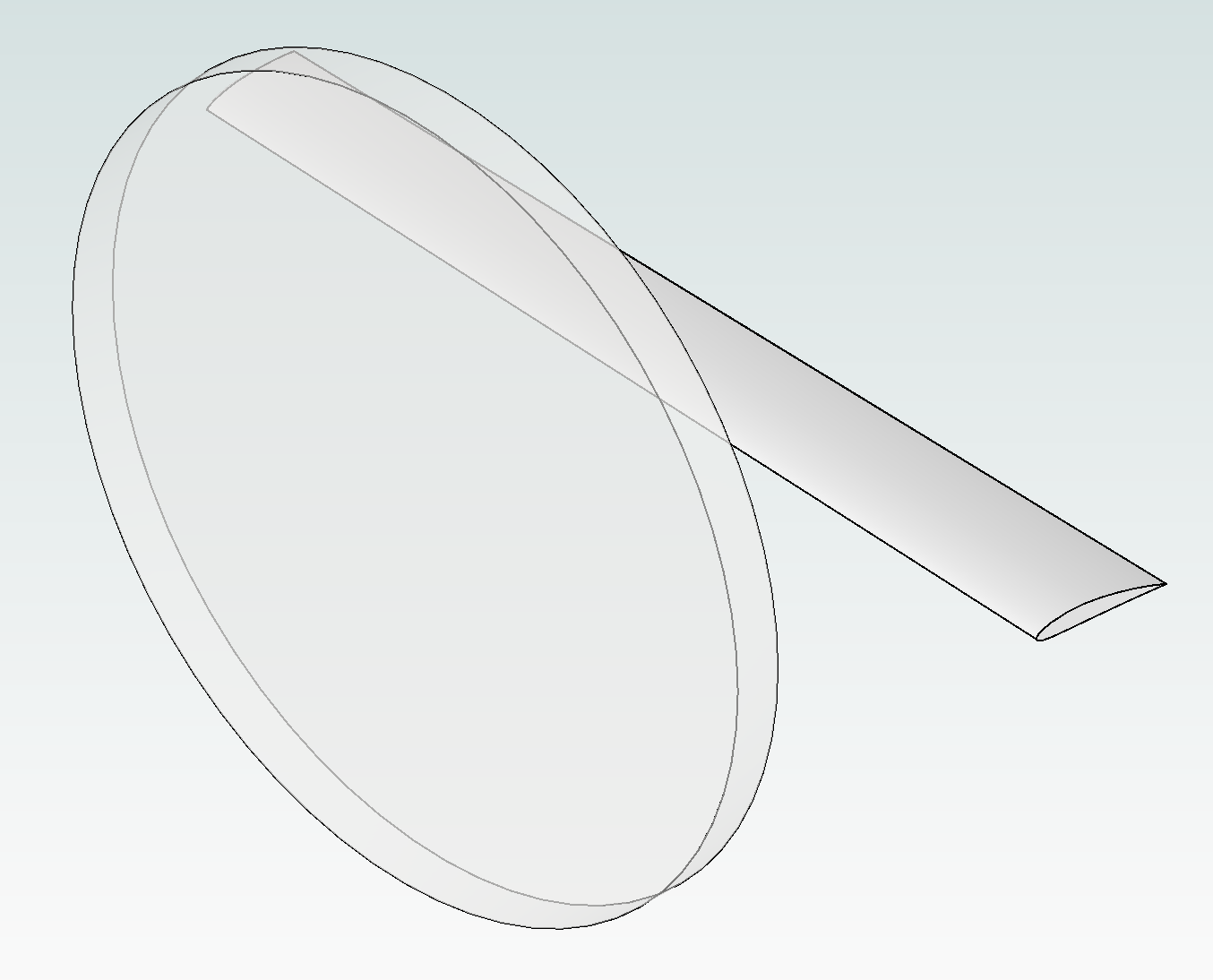
The geometry consists of a BET disk in front of an isolated wing:
Note: The settings in this example are by no means a validation setup; they are crafted to showcase the capabilities of Flow360 and we have intentionally reduced node count and example FC cost. For rigorous validation, modify the settings as needed.
1. Create project from geometry#
We first import the Flow360 Python API, load the BET example files, and create a project from the isolated-wing geometry. This sets up the geometry object we will use for meshing, modeling, and post-processing.
[1]:
import flow360 as fl
from flow360.examples import TutorialBETDisk

TutorialBETDisk.get_files()

project = fl.Project.from_geometry(
    TutorialBETDisk.geometry, name="Tutorial BETDisk from Python"
)
geometry = project.geometry

# show face and edge groupings
geometry.group_faces_by_tag("faceName")
geometry.group_edges_by_tag("edgeName")
[12:12:01] INFO: Geometry successfully submitted:
                   type        = Geometry
                   name        = Tutorial BETDisk from Python
                   id          = geo-25e23e0d-fd3a-4772-90d6-47b912d35eff
                   status      = uploaded
                   project id  = prj-82a38889-787a-4db3-8b46-a6865fda2a58
INFO: Waiting for geometry to be processed.
2. Define BET disk refinements#
Here we define an axisymmetric refinement region around the rotor using a cylindrical volume and AxisymmetricRefinement. The cylinder approximates where the BET disk acts, and the refinement spacings control the local mesh resolution in axial, radial, and circumferential directions. Choosing a cylinder slightly larger than the rotor helps ensure the rotor-affected region is well resolved.
[2]:
with fl.SI_unit_system:
    cylinder1 = fl.Cylinder(
        name="cylinder1",
        axis=[1, 0, 0],
        center=[-2.0, 5.0, 0],
        outer_radius=4.0,
        height=0.6,
    )

    bet_disk_refinement = fl.AxisymmetricRefinement(
        name="BET_Disk",
        spacing_axial=0.02,
        spacing_radial=0.03,
        spacing_circumferential=0.06,
        entities=cylinder1,
    )
[12:12:22] INFO: using: SI unit system for unit inference.
3. Define meshing parameters#
Next we define the global meshing parameters, combining an automatically generated farfield with additional local refinements. A second cylinder provides a region of uniform refinement around the wing and rotor, while the BET disk refinement from the previous step is included to resolve the rotor region. These settings control the overall mesh size, boundary layer resolution, and key refinement zones for the simulation.
[3]:
with fl.SI_unit_system:
    cylinder2 = fl.Cylinder(
        name="cylinder2",
        axis=[1, 0, 0],
        center=[0, 5, 0],
        outer_radius=4.1,
        height=5,
    )
    farfield = fl.AutomatedFarfield()
    meshing_params = fl.MeshingParams(
        defaults=fl.MeshingDefaults(
            surface_max_edge_length=0.5,
            boundary_layer_growth_rate=1.15,
            boundary_layer_first_layer_thickness=1e-06,
        ),
        volume_zones=[farfield],
        refinements=[
            bet_disk_refinement,
            fl.UniformRefinement(
                name="cylinder_refinement", spacing=0.1, entities=[cylinder2]
            ),
        ],
    )
INFO: using: SI unit system for unit inference.
4. Define BET disk model#
The BET disk model is defined from an xrotor file. This file contains a 2D database of drag, lift and moment coefficients of the airfoils used in the blades depending on Reynolds and Mach numbers.
Download XROTOR file to get the file used in this tutorial so you can inspect its structure. A detailed explanation of the xrotor translation tool is written in BET translators.
In the next code cell we will:
Define a cylindrical volume that approximates the physical rotor disk where the BET forces will be applied.
Load the XROTOR file using a dedicated
fl.XROTORFilehelper so Flow360 can interpret the aerodynamic tables.Build a
fl.BETDiskmodel from the XROTOR data and specify the rotor operating conditions (rotation direction, rotational speed, reference chord, number of loading nodes, and units).
This BET model will later be attached to the simulation as one of the physical models in the models list.
[4]:
with fl.SI_unit_system:
    bet_cylinder = fl.Cylinder(
        name="bet_cylinder",
        axis=[-1, 0, 0],
        center=[-2.0, 5.0, 0.0],
        outer_radius=3.81,
        height=0.4572,
    )

    xrotor_file = fl.XROTORFile(file_path=TutorialBETDisk.extra["xrotor"])
    bet_disk_model = fl.BETDisk.from_xrotor(
        file=xrotor_file,
        rotation_direction_rule="rightHand",
        omega=460 * fl.u.rpm,
        chord_ref=0.3556,
        n_loading_nodes=20,
        entities=bet_cylinder,
        angle_unit=fl.u.deg,
        length_unit=fl.u.m,
    )
INFO: using: SI unit system for unit inference.
5. Define SimulationParams#
We now collect all inputs into a single fl.SimulationParams object. This includes the meshing setup, reference geometry, operating condition, and steady-state time-stepping. We also specify the physical and boundary models (walls, farfield, symmetry, fluid solver, and the BET disk) and choose which volume and surface quantities to output for later analysis.
[5]:
with fl.SI_unit_system:
    params = fl.SimulationParams(
        meshing=meshing_params,
        reference_geometry=fl.ReferenceGeometry(
            moment_center=[0.375, 0, 0],
            moment_length=[1.26666666, 1.26666666, 1.26666666],
            area=12.5,
        ),
        operating_condition=fl.AerospaceCondition.from_mach(
            mach=0.182,
            alpha=5 * fl.u.deg,
            reference_mach=0.54,
        ),
        time_stepping=fl.Steady(
            max_steps=10000, CFL=fl.RampCFL(initial=1, final=100, ramp_steps=2000)
        ),
        models=[
            fl.Wall(
                surfaces=[
                    geometry["wing"],
                    geometry["tip"],
                ],
            ),
            fl.Freestream(surfaces=farfield.farfield),
            fl.SlipWall(surfaces=farfield.symmetry_planes),
            fl.Fluid(
                navier_stokes_solver=fl.NavierStokesSolver(
                    absolute_tolerance=1e-12,
                ),
                turbulence_model_solver=fl.SpalartAllmaras(
                    absolute_tolerance=1e-10,
                    update_jacobian_frequency=1,
                    equation_evaluation_frequency=1,
                ),
            ),
            bet_disk_model,
        ],
        outputs=[
            fl.VolumeOutput(
                output_fields=[
                    "primitiveVars",
                    "betMetrics",
                    "qcriterion",
                ],
            ),
            fl.SurfaceOutput(
                surfaces=geometry["*"],
                output_fields=[
                    "primitiveVars",
                    "Cp",
                    "Cf",
                    "CfVec",
                ],
            ),
        ],
    )
INFO: using: SI unit system for unit inference.
6. Run case#
We now launch the simulation case from the project using the SimulationParams we assembled. The returned case object will be used to monitor the run and access results for post-processing.
[6]:
case = project.run_case(
    params=params, name="Case of tutorial BETDisk from Python", use_beta_mesher=True
)
INFO: using: SI unit system for unit inference.
[12:12:24] INFO: Selecting beta/in-house mesher for possible meshing tasks.
[12:12:26] INFO: Successfully submitted:
                   type        = Case
                   name        = Case of tutorial BETDisk from Python
                   id          = case-806e077b-b493-47ce-b776-9a4f5ef46290
                   status      = pending
                   project id  = prj-82a38889-787a-4db3-8b46-a6865fda2a58
7. Post-processing#
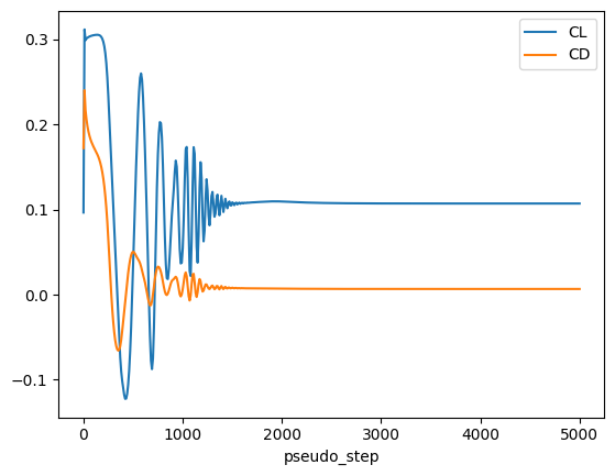
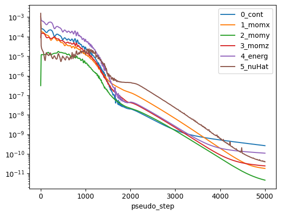
Finally, we wait for the case to finish, read the results, and make a few simple plots. We look at the evolution of integrated lift and drag coefficients and the nonlinear residuals to assess convergence and overall solution quality.
[7]:
import matplotlib.pyplot as plt

case.wait()
results = case.results

total_forces = results.total_forces.as_dataframe()
total_forces.plot("pseudo_step", ["CL", "CD"])

non_linear = results.nonlinear_residuals.as_dataframe()
non_linear.plot(
    "pseudo_step",
    ["0_cont", "1_momx", "2_momy", "3_momz", "4_energ", "5_nuHat"],
    logy=True,
)
plt.show()
[12:23:48] INFO: Saved to /tmp/tmpri5txw3w/3bd23e60-41af-4f9b-bfcd-a106345e2575.csv
[12:23:50] INFO: Saved to /tmp/tmpri5txw3w/4bf86786-76f5-4e18-94a0-2cfe0d4b5a35.csv