Flat Plate with Structural Aerodynamic Load#
In this example, we present an illustrative case where a flat plate rotates while being subjected to a rotational spring moment and damper as well as aerodynamic loads. The structural dynamics are modeled by a torsional spring–mass–damper ODE driven by the aerodynamic pitching moment \(\tau_y(t)\):
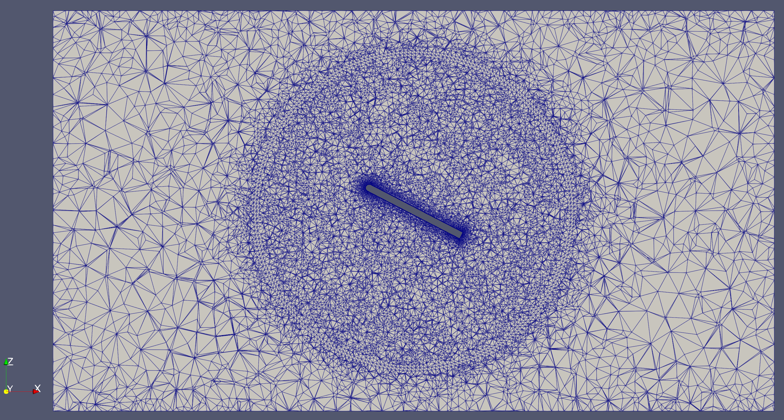
As you can see below, the flat-plate mesh consists of two zones separated by a circular sliding interface. The inner zone will rotate while the outer zone remains stationary. This is the same mesh topology as what is used for rotating propeller simulations.
Note: The settings in this example are by no means a validation setup; they are crafted to showcase the capabilities of Flow360 and we have intentionally reduced node count and example FC cost. For rigorous validation, modify the settings as needed.
1. Imports and Create Project#
In this section we:
Import Flow360 and NumPy:
flow360provides the high-level Python API for setting up and running the CFD case, whilenumpyis used for basic math and unit handling.Load the flat-plate mesh: the CGNS file
rotatingPlate.cgnsis uploaded to the Flow360 platform and becomes the basis of theProject.Create a
ProjectandVolumeMeshhandle:Project.from_volume_mesh(mesh)creates (or reuses) a project on the server, andvm = project.volume_meshgives convenient access to mesh blocks and boundary entities used later for BCs and UDD setup.
[1]:
import flow360 as fl
from flow360.examples import TutorialUDDStructural
import numpy as np

TutorialUDDStructural.get_files()
project = fl.Project.from_volume_mesh(
    TutorialUDDStructural.mesh_filename, name="UDD structural tutorial from Python"
)
vm = project.volume_mesh
[18:39:40] INFO: VolumeMesh successfully submitted:
                   type        = Volume Mesh
                   name        = UDD structural tutorial from Python
                   id          = vm-b11bca1f-a264-487c-8f1a-eeb168096f2c
                   status      = uploaded
                   project id  = prj-50ef37d8-4b77-480e-92c1-98a68f613176
2. Operating Conditions#
Since the mesh flat plate length is different from experiment, the operating conditions are computed based on a reference Mach number and reference Reynolds number.
More precisely, the code below:
Defines experimental reference values: freestream velocity, reference length, density, temperature, and kinematic viscosity are specified in SI units using Flow360’s unit helpers.
Computes Mach and Reynolds numbers:
Machis derived fromu_infand the speed of sound;Reynoldsis based on the experiment reference length and kinematic viscosity.Maps to mesh units:
Re_mesh_unitrescales the Reynolds number to the mesh length scale so the simulation matches the intended experimental conditions.Creates an
AerospaceCondition:operating_condition = fl.AerospaceCondition.from_mach_reynolds(...)packages these quantities into a reusable object for the solver.
[2]:
# Experiment reference values in SI unit system
u_inf = 15 * fl.u.m / fl.u.s
ref_length = (4 * fl.u.inch).to("m")
ref_density = 1.226 * fl.u.kg / fl.u.m**3
ref_T = 288.15 * fl.u.K
kinematic_viscosity = 14.61e-6 * fl.u.m**2 / fl.u.s

R = 287.058 * fl.u.J / (fl.u.kg * fl.u.K)
speed_of_sound = np.sqrt(1.4 * R * ref_T).to("m/s")
Mach = u_inf / speed_of_sound
Reynolds = u_inf * ref_length / kinematic_viscosity

# Define operating condition based on reference values
mesh_unit = project.length_unit
Re_mesh_unit = Reynolds * mesh_unit.to_value() / ref_length
operating_condition = fl.AerospaceCondition.from_mach_reynolds(
    mach=Mach,
    reynolds_mesh_unit=Re_mesh_unit,
    project_length_unit=project.length_unit,
)
[18:39:58] INFO: Density and viscosity were calculated based on input data, ThermalState will be automatically
           created.
2. Boundary Conditions and Rotating Interfaces#
The following cell defines how the flow interacts with the flat plate and how the inner plate region is allowed to rotate:
Freestream and walls:
Freestreamis applied on the far-field block,SlipWallon non-plate walls, andWall(no-slip) on the plate itself.Rotating volume:
volume_rotation = vm["plateBlock"]selects the inner block that will move as a rigid body around the specified axis.Rotation model:
fl.Rotation(..., spec=fl.FromUserDefinedDynamics())tells Flow360 that the rotational motion will be driven by a User Defined Dynamic (UDD) law defined later, rather than by a prescribed constant rate. The UDD will specify \(\dot{\omega}\), \(\omega\), and \(\theta\) for each physical step.
[3]:
# Boundary Conditions
freestream = fl.Freestream(entities=vm["farFieldBlock/farField"])
slip_wall = fl.SlipWall(entities=vm["*/slipWall"])
no_slip_wall = fl.Wall(entities=vm["plateBlock/noSlipWall"])
BCs = [freestream, slip_wall, no_slip_wall]

# Rotating zones
volume_rotation = vm["plateBlock"]
volume_rotation.center = (0, 0, 0) * fl.u.m
volume_rotation.axis = [0, 1, 0]
rotation_model = fl.Rotation(
    entities=[volume_rotation], spec=fl.FromUserDefinedDynamics()
)
3. Couple Structural Model#
The dynamics of the plate will be influenced by the spring and damper according to this law:
Symbol |
Description |
|---|---|
\(\theta\) |
Rotation angle of the plate in radians. |
\(\omega\) |
Rotation velocity of the plate in radians. |
\(\dot{\omega}\) |
Rotation acceleration of the plate in radians. |
\(\tau_y\) |
Aerodynamic moment exerted on the plate. |
\(K\) |
Stiffness of the spring attached to the plate at the structural support. |
\(\zeta\) |
Structural damping ratio. |
\(\omega_N\) |
Structural natural angular frequency. |
\(I\) |
Structural moment of inertia. |
In the next few cells we will:
Specify numerical values for the structural parameters (\(I, \zeta, K, \omega_N, \theta_0\)) and initial conditions for \(\theta\) and \(\dot{\omega}\).
Set the time step and number of steps so that the structural oscillations are resolved in time.
Encode this ODE system as a User Defined Dynamic in Flow360, which takes the aerodynamic moment \(\tau_y\) as input and outputs the plate rotation state used by the mesh motion model.
3.1 Define Model Constants#
Here we choose the numerical values that define the torsional spring–mass–damper model of the plate:
\(I\): structural moment of inertia of the rotating plate about its hinge axis.
\(\zeta\): non-dimensional structural damping ratio; smaller values lead to slowly decaying oscillations.
\(\theta_0\): equilibrium pitch angle about which the spring tries to restore the plate.
iniPert: initial perturbation added on top of \(\theta_0\), which directly sets the initial oscillation amplitude.\(K\) and \(\omega_N\): linear torsional stiffness and corresponding natural frequency, related approximately by \(\omega_N = \sqrt{K/I}\).
initThetaandinitOmegaDot: initial angle and angular acceleration used to initialize the UDD state vector for the first physical time step.
[4]:
deg2rad = np.pi / 180

I = 0.443768309310345  # Structural moment of inertia
zeta = 0.005  # Structural damping ratio
theta0 = 5 * deg2rad  # Initial equilibrium angle
iniPert = 45 * deg2rad  # Initial perturbation
K = 0.005  # Stiffness of the spring
omegaN = np.sqrt(K / I)  # Structural natural angular frequency
initTheta = theta0 + iniPert
initOmegaDot = (0 - K * (initTheta - theta0)) / I
3.2 Define Time Settings#
The next cell configures the unsteady time marching for the coupled aeroelastic simulation:
deltaNonDimensional: a non-dimensional time step size, scaled by the acoustic time based onref_length / speed_of_sound.delta_SI: the corresponding physical time step in seconds, passed to the solver asstep_size.n_steps: total number of physical steps to march the coupled flow–structure system.fl.Unsteady(...): creates a time stepping object that controls the outer physical time loop and the number of inner pseudo-steps used to converge each time level.
[5]:
deltaNonDimensional = 0.5
delt_SI = deltaNonDimensional * (ref_length / speed_of_sound)
n_steps = 3000
time_stepping = fl.Unsteady(
    max_pseudo_steps=100,
    step_size=delt_SI,
    steps=n_steps,
)
3.3 UDD for structural solver#
This User Defined Dynamic (UDD) encodes the structural ODE and couples it to the CFD solution:
Inputs:
momentYis the aerodynamic pitching moment from the wall patch on the plate.Constants: the structural parameters (
I,zeta,K,omegaN,theta0) are passed in once and reused each step.Output Vars: the state vector
state[0:3]stores \(\dot{\omega}\), \(\omega\), and \(\theta\); these are exposed asomegaDot,omega, andthetaoutputs. It is important to use this names since the values of \(\dot{\omega}\), \(\omega\), and \(\theta\) will be updated forstate[0:3]for each physical step, this will drive the rotation of the sliding interface.Initial values:
state_vars_initial_valueinitializes the ODE withinitOmegaDotandinitThetafrom Section 3.1.Update law: for each physical step (
pseudoStep == 0), the first expression integrates \(\dot{\omega}\), the second integrates \(\omega\), and the third integrates \(\theta\) using an explicit Euler update withtimeStepSize.Coupling to motion:
output_target=vm["plateBlock"]sends the updatedthetaback to the rotating volume, which the rotation model uses to move the mesh.
[6]:
dynamic = fl.UserDefinedDynamic(
    name="dynamicTheta",
    input_vars=["momentY"],
    constants={
        "I": I,
        "zeta": zeta,
        "K": K,
        "omegaN": omegaN,
        "theta0": theta0,
    },
    output_vars={
        "omegaDot": "state[0];",
        "omega": "state[1];",
        "theta": "state[2];",
    },
    state_vars_initial_value=[str(initOmegaDot), "0.0", str(initTheta)],
    update_law=[
        "if (pseudoStep == 0) (momentY - K * ( state[2] - theta0 ) - 2 * zeta * omegaN * I *state[1] ) / I; else state[0];",
        "if (pseudoStep == 0) state[1] + state[0] * timeStepSize; else state[1];",
        "if (pseudoStep == 0) state[2] + state[1] * timeStepSize; else state[2];",
    ],
    input_boundary_patches=vm["plateBlock/noSlipWall"],
    output_target=vm["plateBlock"],
)
4. Outputs#
We will put some slice outputs to have a time visualisation of the flowfield.
The code below configures what Flow360 writes during the run:
SliceOutput: extracts a 2D slice at \(y=0\) (normal to the \(y\) axis) at selected time steps, outputting primitive variables and Mach number in Tecplot format.VolumeOutput: writes 3D volume fields (primitive variables, \(Q\)-criterion, and Mach number) for full-flow visualization.Output frequency:
frequencyandfrequency_offsetcontrol how often and when in the run the slice output is written, so that the transient behavior of the oscillating plate can be visualized efficiently.
[7]:
with fl.SI_unit_system:
    outputs = [
        fl.SliceOutput(
            slices=[fl.Slice(name="y-slice", origin=(0, 0, 0), normal=(0, 1, 0))],
            output_format=["tecplot"],
            output_fields=["primitiveVars", "Mach"],
            frequency=10,
            frequency_offset=200,
        ),
        fl.VolumeOutput(
            output_format=["tecplot"],
            output_fields=["primitiveVars", "qcriterion", "Mach"],
        ),
    ]
INFO: using: SI unit system for unit inference.
5. Simulation Parameters#
The previous defined settings are used here to define the SimulationParams.
Specifically, this section:
Defines a reference geometry: sets the aerodynamic reference moment center, length, and area used to non-dimensionalize forces and moments.
Attaches the operating condition and time stepping:
operating_conditionandtime_steppingfrom earlier sections are plugged into the top-level parameters.Configures fluid and turbulence solvers: creates a
NavierStokesSolverandSpalartAllmarasturbulence model with tolerances, linear solver controls, and accuracy/order settings tailored to this case.Adds models and BCs: combines all boundary conditions, the rotation model, and the User Defined Dynamic into the list of active models.
Registers outputs: passes the
outputslist so that slice and volume data are produced according to the configuration in Section 4.
[8]:
with fl.SI_unit_system:
    param = fl.SimulationParams(
        reference_geometry=fl.ReferenceGeometry(
            moment_center=(0, 0, 0),
            moment_length=(1, 1, 1) * mesh_unit,
            area=0.5325 * mesh_unit * mesh_unit,
        ),
        operating_condition=operating_condition,
        time_stepping=time_stepping,
        models=[
            fl.Fluid(
                navier_stokes_solver=fl.NavierStokesSolver(
                    absolute_tolerance=1e-9,
                    relative_tolerance=1e-3,
                    linear_solver=fl.LinearSolver(max_iterations=35),
                    kappa_MUSCL=0.33,
                    order_of_accuracy=2,
                    update_jacobian_frequency=1,
                    equation_evaluation_frequency=1,
                    low_mach_preconditioner=True,
                ),
                turbulence_model_solver=fl.SpalartAllmaras(
                    absolute_tolerance=1e-8,
                    relative_tolerance=1e-2,
                    linear_solver=fl.LinearSolver(max_iterations=35),
                    order_of_accuracy=2,
                    rotation_correction=True,
                    update_jacobian_frequency=1,
                    reconstruction_gradient_limiter=0.5,
                    equation_evaluation_frequency=1,
                ),
            ),
            *BCs,
            rotation_model,
        ],
        outputs=outputs,
        user_defined_dynamics=[dynamic],
    )
INFO: using: SI unit system for unit inference.
6. Run Case#
Here we finally submit the configured simulation to Flow360:
project.run_case(param): packages the mesh, models, operating condition, and solver settings into aCaseand sends it to the server.case: can be used to monitor status, wait for completion, and fetch results (as done in the post-processing section).
[9]:
case = project.run_case(params=param, name="UDD structural tutorial from Python")
           INFO: Density and viscosity were calculated based on input data, ThermalState will be automatically
           created.
INFO: using: SI unit system for unit inference.
[18:40:00] INFO: Successfully submitted:
                   type        = Case
                   name        = UDD structural tutorial from Python
                   id          = case-cb351231-8428-4b41-8e00-a00cb4c9c61c
                   status      = pending
                   project id  = prj-50ef37d8-4b77-480e-92c1-98a68f613176
7. Post Processing#
Once the case has finished, we read back and visualize key integrated quantities from the server-side results:
Wait for completion:
case.wait()blocks until the CFD run finishes.Total forces:
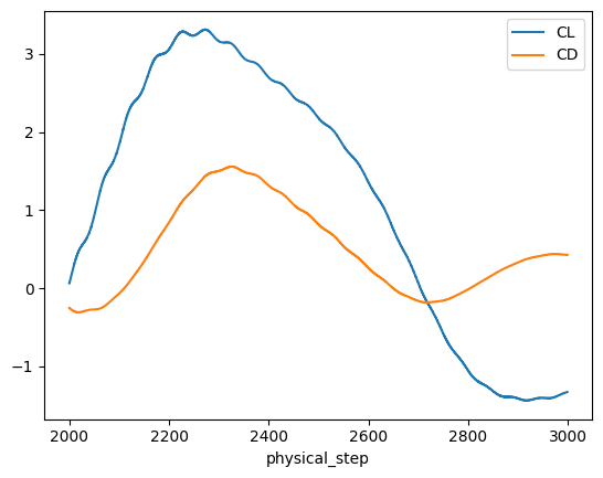
results.total_forces.as_dataframe()returns time histories of lift and drag coefficients (CL,CD), which are plotted versusphysical_stepto show the plate’s oscillatory response.Nonlinear residuals:
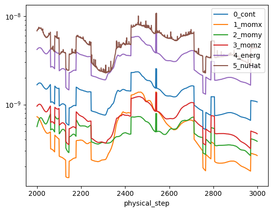
results.nonlinear_residualsexposes solver convergence histories (continuity, momentum, energy, and turbulence variable), plotted on a log scale to verify converge. The data is filtered to show only the last pseudo step usingfilter_physical_steps_only.
[10]:
import matplotlib.pyplot as plt

case.wait()

results = case.results

total_forces = results.total_forces.as_dataframe()
total_forces_2000 = total_forces[total_forces["physical_step"] >= 2000]
total_forces_2000.plot("physical_step", ["CL", "CD"])

non_linear = results.nonlinear_residuals
non_linear.filter_physical_steps_only()
non_linear = non_linear.as_dataframe()
non_linear_2000 = non_linear[non_linear["physical_step"] >= 2000]
non_linear_2000.plot(
    "physical_step",
    ["0_cont", "1_momx", "2_momy", "3_momz", "4_energ", "5_nuHat"],
    logy=True,
)

plt.show()
[18:58:49] INFO: Saved to /tmp/tmpbfsct6q_/8f1619f2-d54b-48c7-b87b-c4b1cd54fa42.csv
[18:58:51] INFO: Saved to /tmp/tmpbfsct6q_/2715dda5-2f01-4200-a74c-b33fbb253b90.csv