UDD Alpha Controller (Constant CL)#
In this tutorial the UserDefinedDynamic will be used to implement a PI controller that manipulates the angle of attack to achieve a constant given lift coefficient. The project will be started from an example volume mesh and basic python post-processing of the results will be showcased.
1. Imports and Project creation#
At first the flow360 library must be imported.
Note: The settings in this example are by no means a validation setup; they are crafted to showcase the capabilities of Flow360 and we have intentionally reduced node count and example FC cost. For rigorous validation, modify the settings as needed.
[1]:
import flow360 as fl
from flow360.examples import OM6wing
Then the Project has to be created. In this case it will be started from the volume mesh.
[2]:
OM6wing.get_files()

project = fl.Project.from_volume_mesh(
    OM6wing.mesh_filename, name="Tutorial UDD alpha controller from Python"
)
[15:27:34] WARNING: The expected mapbc file
           c:\Code\Flow360Documentation\.venv\Lib\site-packages\flow360\examples\om6wing\wing_tetra.1.mapbc
           specifying user-specified boundary names doesn't exist.
[15:27:46] INFO: VolumeMesh successfully submitted:
                   type        = Volume Mesh
                   name        = Tutorial UDD alpha controller from Python
                   id          = vm-70f5a518-3df9-49f1-9b3e-a4d6c5a5a04e
                   status      = uploaded
                   project id  = prj-52037feb-d308-4ee7-ab53-d7163a45358f
The project can also be referenced by its unique ID if it was already created.
[3]:
# project = fl.Project.from_cloud(project_id="prj-your_id_here")
The Project entity stores all of the information about the root asset it was created from such as boundary names.
[4]:
volume_mesh = project.volume_mesh

print("Volume mesh boundaries:")
for boundary in volume_mesh.boundary_names:
    print(f"  - {boundary}")
Volume mesh boundaries:
  - 3
  - 1
  - 2
2. Setting up the base of SimulationParams#
As the project is started from the volume mesh, the meshing part is not required. The basic case setup consists of:
setting appropriate operating conditions in
operating_condition,specifying the reference values for coefficient calculation in
reference_geometry,choosing between the transient vs a steady simulation in
time_stepping,setting appropriate boundary conditions in the
modelssection,specifying wanted outputs in
outputs.
The operating_condition is set using a given Reynolds number and Mach.
[5]:
with fl.SI_unit_system:
    operating_condition = fl.AerospaceCondition.from_mach_reynolds(
        reynolds_mesh_unit=11.72e6,
        mach=0.84,
        project_length_unit=0.80167 * fl.u.m,
        temperature=297.78,
        alpha=3.06 * fl.u.deg,
        beta=0 * fl.u.deg,
    )
[15:28:04] INFO: using: SI unit system for unit inference.
[15:28:05] INFO: Density and viscosity were calculated based on input data, ThermalState will be automatically
           created.
The reference_geometry is set according to the input geometry and time_stepping is set to Steady.
[6]:
with fl.SI_unit_system:
    reference_geometry = fl.ReferenceGeometry(
        area=1.15315,
        moment_center=[0, 0, 0],
        moment_length=[1.47601, 0.80167, 1.47601],
    )
    time_stepping = fl.Steady(
        max_steps=2000,
    )
INFO: using: SI unit system for unit inference.
The boundary conditions are assigned to given volume mesh boundaries by specifying them in the models section.
[7]:
with fl.SI_unit_system:
    models = [
        fl.Wall(surfaces=[volume_mesh["1"]]),
        fl.SlipWall(surfaces=[volume_mesh["2"]]),
        fl.Freestream(surfaces=[volume_mesh["3"]]),
    ]
INFO: using: SI unit system for unit inference.
For the outputs basic SurfaceOutput is specified focusing on the pressure coefficient and the wall shear stress.
[8]:
with fl.SI_unit_system:
    outputs = [
        fl.SurfaceOutput(
            surfaces=volume_mesh["1"],
            output_fields=[
                "Cp",
                "Cf",
                "CfVec",
                "yPlus",
            ],
        )
    ]
INFO: using: SI unit system for unit inference.
Finally all the fields can be input into the SimulationParams class that is used as a setup data source for the simulation.
[9]:
with fl.SI_unit_system:
    params = fl.SimulationParams(
        operating_condition=operating_condition,
        reference_geometry=reference_geometry,
        time_stepping=time_stepping,
        models=models,
        outputs=outputs,
    )
INFO: using: SI unit system for unit inference.
3. Adding UserDefinedDynamic#
The goal of the UserDefinedDynamic object will be to “search” for a specified angle of attach for which the lift coefficient of the wing is a certain value (0.4 in this case). To achieve that the PI controller will be used to update the value of the alpha variable in each pseudo_step.
The UserDefinedDynamic requires the specification of a few parameters:
nameis the name of the dynamic, will be used to access the variables present in it in post-processing,input_varsis the list of variables from the solution that will be used in calculations ,constantsare the predefined constants used in calculations, in this case those include the CL target and PI controller constants,output_varsare the variables in the case that are controlled, they are defined using a dictionary where the key is the name of the controlled variable and the value is a formula using the predefined constants, state variables or solution variables such aspseudo_step; the formula should be written using C syntax,state_vars_initial_valuedefine initial values of the state variables, in this case the initial state ofstate[0]is thealphaAngleand the initial state ofstate[1]is0.0,update_lawis a list of expression used to calculate the state variables in eachpseudo_stepthose expressions also should use C syntax,input_boundary_patchesis a list of boundaries that are used in the calculation of theinput_varsmeaning theCLused for calculation will be only taken from thevolume_mesh["1"]boundary.
The PI controller in this case is formulated so that it does not turn on until 500 pseudo steps, which allows the simulation to converge initially before applying corrections. After this number of steps the state[0] calculates the new alphaAngle to set and state[1] gets the numerical integral part of the controller.
The state is a vector of values that can be referenced in the expressions and is updated at each step according to update_law.
[10]:
alpha_controller = fl.UserDefinedDynamic(
    name="alphaController",
    input_vars=["CL"],
    constants={"CLTarget": 0.4, "Kp": 0.2, "Ki": 0.002},
    output_vars={"alphaAngle": "if (pseudoStep > 500) state[0]; else alphaAngle;"},
    state_vars_initial_value=["alphaAngle", "0.0"],
    update_law=[
        "if (pseudoStep > 500) state[0] + Kp * (CLTarget - CL) + Ki * state[1]; else state[0];",
        "if (pseudoStep > 500) state[1] + (CLTarget - CL); else state[1];",
    ],
    input_boundary_patches=[volume_mesh["1"]],
)
params.user_defined_dynamics = [alpha_controller]
4. Running the simulation#
The simulation is then run using the run_case function of the Project.
[11]:
case = project.run_case(
    params=params, name="Case of tutorial UDD alpha controller from Python"
)
           INFO: Density and viscosity were calculated based on input data, ThermalState will be automatically
           created.
INFO: using: SI unit system for unit inference.
[15:28:07] INFO: Successfully submitted:
                   type        = Case
                   name        = Case of tutorial UDD alpha controller from Python
                   id          = case-79b42c52-01a4-44fd-b410-3c6c67082df0
                   status      = pending
                   project id  = prj-52037feb-d308-4ee7-ab53-d7163a45358f
5. Post-processing#
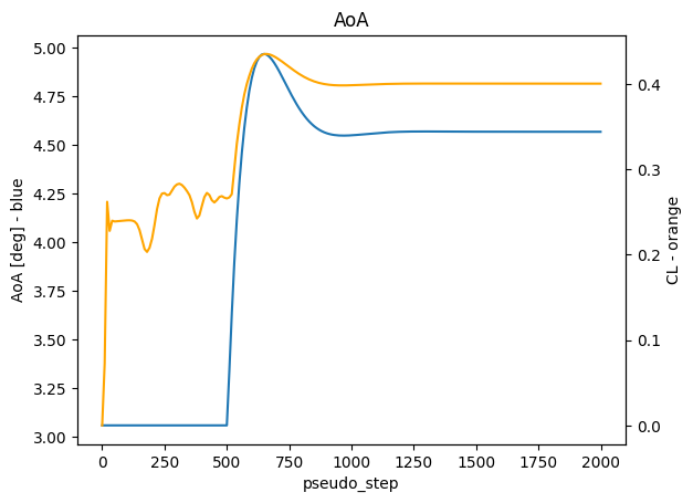
To access the results of the simulation it has to be finished. They can be found in the results parameter. Below the state of the controller and calculated alpha is plotted.
[12]:
case.wait()

udd_data = case.results.user_defined_dynamics["alphaController"]

ax0 = udd_data.as_dataframe().plot(
    x="pseudo_step",
    y="alphaAngle",
    title="AoA",
    ylabel="AoA [deg] - blue",
    legend=False,
)
ax1 = ax0.twinx()
udd_data.as_dataframe().plot(
    x="pseudo_step", y="CL", ylabel="CL - orange", ax=ax1, color="orange", legend=False
)
[15:29:27] INFO: Saved to C:\Users\user\AppData\Local\Temp\tmpvdihtq8f\1eba06e3-b226-42da-9f23-b992ec6362e3.csv
[12]:
<Axes: xlabel='pseudo_step', ylabel='CL - orange'>
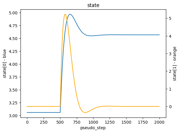
[13]:
ax0 = udd_data.as_dataframe().plot(
    x="pseudo_step", y="state[0]", title="state", ylabel="state[0] - blue", legend=False
)
ax1 = ax0.twinx()
udd_data.as_dataframe().plot(
    x="pseudo_step",
    y="state[1]",
    ylabel="state[1] - orange",
    ax=ax1,
    color="orange",
    legend=False,
)
[13]:
<Axes: xlabel='pseudo_step', ylabel='state[1] - orange'>